A ship’s propeller likely did this damage to the dorsal fin of a female northern resident killer whale (A1) known as “Stubbs” (well prior to her death in 1974).
Most folks think that killer whales — top predators of the ocean — are too fast and smart to get hit by big ships. But, if you look back through the history of salmon-seeking orcas over decades of growing human population and vessel traffic, a long list of injury and death reveals that they are sometimes struck by big ships (as well as by small boats), including within the Salish Sea. The starkest example is a collision in 1973 with a B.C. ferry that killed a young orca.
The Comox ferry incident (1973)
A clear case in which a ferry in B.C. struck a resident orca was an incident described in the 2nd edition of a book called “Killer Whales” (Ford et al., 2000; see excerpt below & this photo album with the relevant pages). On 26 December 1973, en route from Comox on Vancouver Island to Powell River on the BC mainland (see #17 on the map below), the BC Ferry “M/V Comox” struck a juvenile northern resident killer whale (A21).
No whales were sighted prior to the collision of the orca and the ship’s propeller, but conditions are rarely optimal for marine mammal observers in the northern Strait of Georgia in late December. The Captain noted that there was a lot of debris in the water that day. And based on the hourly weather report that day in 1973 (see below), there was some rain in the morning, and by late afternoon (3:45 pm) it was overcast with rising light winds, probably resulting in some chop.
It was also late in the day, that close to the winter solstice (December 21). According to a sunset calculator, that Wednesday the sun set at 16:24, just ~45 minutes after the strike occurred. Since the ferry was bound for Powell River (heading west-northwest), any low-angle sunlight would have been coming over the port stern quarter, making visibility in that direction more difficult. Some direct light from the setting sun slipping under the overhead clouds seems likely given that the winds were out of the west that afternoon and evening, and the skies cleared some 4 hours later. In any case, in the direction the ferry was headed (to the east) there was no backlighting from the sun — a situation which often makes killer whale blows much easier to see at a distance.
An example of how back-lighting can reveal orcas, especially when there’s a dark background or rough water. (Credit: Barbara Bender, All Aboard Sailing)
Somehow, the Captain and crew failed to observe the 4 killer whales until after the impact of one of the two calves with the propeller was heard. Maybe visibility was too low, maybe they were distracted (they mention conversing at the time), or maybe the orcas converged from an aft quarter hidden by the glare of the setting sun. What was observed when the ferry returned to the scene was a lot of blood in the water, propeller lacerations along the injured orca’s flank, and the parents trying to keep their calf upright.
The Captain assumed that the injured orca would soon die and the ferry continued on to Powell River. Surprisingly, it was observed 15 days later, still being assisted by its parents. This is another example of the persistent, strong bonds in orca families, and the duration of the parent’s efforts bears an uncanny resemblance to the 17-day “tour of grief” by J35 with her dead calf last summer. Unfortunately, A21 was never sighted again, so we can safely conclude that the collision was fatal.
That’s the strongest evidence that salmon-seeking orcas are sometimes killed by big ships within the Salish Sea, in this case specifically by a BC Ferry. But there are many other strikes of orcas that have been documented in BC and Washington State (e.g. Williams & O’Hara, 2010). Here is a working list of vessel strikes on killer whales, as well as other cetaceans, in the region:
The case of southern resident killer whale J34 (2016)
The most recent possible strike of a fish-eating killer whale is the stranding of J34 (aka “Doublestuf”) an adult male endangered southern resident discovered floating dead just north of Vancouver, BC, in December, 2016. While all available information about the death of J34 is currently insufficient to determine the cause of the “blunt force trauma” that killed him, the most parsimonious interpretation is that he was struck by a vessel.
The hypothesis that J34 was killed by a vessel was proposed very early in the DFO response to the incident. Just a day after J34’s body had been towed to a beach near Sechelt for a necropsy, DFO Pacific Region Marine Mammal Coordinator Paul Cottrell said in an interview with CTV (at 1:00): “Vessel strike could be a potential… and something we’ll be investigating going forward.”
That investigation has been on-going for 2.5 years now, with no final necropsy report available to the public and scientists. Such a report typically would contain important information about the health of the animal prior to injury, condition of the carcass, the mechanisms of injuries, and the most probable cause(s) of death. Beam Reach has made multiple requests for the report, but only a summary has been released. It’s starting to seem like science is being suppressed by some part of the Canadian Government well above the dedicated mariners, First Nations volunteers, and scientists who recovered the body and undertook a prompt, thorough necropsy and many important follow-up investigations, like a CAT scan of the skull to look for fractures, as well as tissue and blood analyses. It likely contains information that should be considered in important on-going conservation processes — like Canada’s Technical Working Groups and the environmental reviews of both the Transmountain pipeline and Roberts Bank container ship terminal expansions.
But even without the final necropsy report, under the assumption that J34 was struck by a vessel, we can make some initial inferences about what type of vessel it was. Here’s a synopsis of what we know and can infer:
The location of J34 floating just south of the Trail Islands is established by the AIS/GPS location of the Canadian Coast Guard vessel that towed the body to shore.
The drift of J34 to the point of discovery can be assumed to have been north-northwestward, based on predominant winds (from the south-southeast) measured during the previous week.
This drift direction suggest that vessels that commonly ply routes south of Sechelt would have been most likely to strike J34.
The object responsible for the blunt force trauma suffered by J34 along his side and head was powerful enough to shatter the bone on the inside of his skull, leaving “spicules and sheaves up to 3-4 cm long” within his brain cavity.
By far the most prevalent type of powerful vessel in the direction of drift are the B.C. Ferries that traverse the Strait of Georgia many times per day on three major east-west routes. The closest is the Horseshoe Bay to Departure Bay route, only 20 km to the south of the discovery site (with ~10 transits/day at that time of year, according to the December 2019 schedule)
The spatial relationship of these observations, including the estimated drift direction and inferred (hypothetical) collision sites within B.C. ferry routes are indicated in this static version of the J34 stranding map:
The J34 stranding map with the 3 major B.C. Ferry routes (white dotted lines) that are located south of where J34 was discovered (orange circles) — the direction from which J34 most likely drifted (along the orange line) in the wind and currents prior to his discovery.
The intersection of the ferry routes by a linear extension of the orange drift line occur at about 20, 40, & 70 km, respectively for the Horseshoe Bay – Departure Bay, Tsawwassen – Duke Point, & Tsawwassen – Swartz Bay routes. An important constraint that the final necropsy report could offer is how long J34 had been drifting before he was discovered. All we know now — again from the CTV interview with Paul Cottrell — is that “This animal was very fresh…” With no quantitative estimate of the number of hours or days J34 was adrift, this qualitative condition suggests the the collision could have been local — possibly indicating that the closest ferry route was the most-likely location of a potential strike.
One depiction of the local traffic density in the period just prior to J34’s discovery is this map of AIS tracks:
Archived AIS tracks (from siitech) from a ~1 day period just before J34 was discovered.
Note the typically high traffic density along the routes of the B.C. Ferries, as well as vessel traffic associated with Burrard Inlet in Vancouver. Now take a look at this example of the best information we have about how SRKWs travel into and out of the northern Strait of Georgia during the winter months (Dec – Feb, based on satellite tags deployed by NOAA in 2014 and 2015):
02 Jan 2014 L87 (+J +K pods) satellite tag track
What jumps out at me is that during the winter, they tend to travel north-south while staying west of the commercial shipping lanes. This means that if J34 (in December) was following this pattern, his path would more-likely have crossed the east-west ferry lanes than the shipping lanes associated with Vancouver Island.
A sudden (suspicious?) interest in thermal cameras for BC Ferries
After many years of minimal action on both sides of the border, 2018 witnessed a tremendous acceleration in public and governmental will to help the SRKWs recover. Spurred in part by the global media attention garnered by J35’s tragedy, and catalyzed by a Washington Governor with Presidential aspirations and the political machinations of the Trudeau administration’s Ocean Protection Plan, a wave of new policy developments and investments rolled through the Salish Sea. The wave was propelled in WA by the SRKW Task Force (which met intensively in 2018 along with its Work Groups) while in Canada there were Technical Working Groups hard at work through the winter of 2018-19.
Amid this policy-making maelstrom in the Pacific Northwest, a detail at the very end of this news article from the East Coast of the U.S. made me stop in my tracks and think of J34:
June 13, 2019 Featured Project, WHOI online news & insights
The backstory and motivation of the research project — to avoid “ship strike” — made a lot of sense to me. It was a little ambiguous if by “ship” the young WHOI principal investigator, Dan Zitterbart, meant big vessels like commercial ships, or small vessels like recreational and whale watch boats, or both. But he was at least talking about strikes against the right types of Salish Sea whales: humpbacks, killer whales, etc. Perhaps Dan and the WHOI news editor were just not quite clear about which types of vessels have struck which types of Salish Sea whales in recent decades?
I started to feel a little more cognitive dissonance when I read that WHOI was “working with Transport Canada and B.C. Ferries” (emphasis added), though. “Wait. Why isn’t this a DFO research project?” I thought. “Isn’t DFO being funded through the Ocean Protection Plan for this sort of research?” Esteemed colleagues at DFO like Harald Yurk were quoted, though, arguing that an inter-comparison of thermal imaging and acoustic detection rates would be fruitful. As a coordinator of the Orcasound hydrophone network, this was starting to make good sense again. I began to think that maybe Transport Canada was funding the project and the involvement of the B.C. Ferries was limited to hosting the cameras on Galiano Island at the Sturdies Bay terminal — a site which I know provides a good vantage point for observing the busy summertime SRKW, boat, ship, and ferry traffic at the northeast end of Active Pass.
Cognitive dissonance was abating for me at this point in the article, because I knew that Paul Cottrell of DFO had put an enormous effort in improving DFO’s internal acoustic detection capabilities in the Gulf Islands and beyond. Plus, the article mentioned one of the DFO hydrophones being co-located with the camera study site.
But then, at the very end of the article, came the zinger. Dan was quoted as saying:
if the detection is effective enough, we could eventually think about mounting infrared cameras directly on the bow of ferry ships and having a real-time feedback loop where mariners are alerted to slow down if whales are present
Why would a young investigator from Massachusetts volunteer that his advanced automated detection system should specifically be mounted “on the bow of ferry ships” as opposed to vessels in general? I can only surmise that B.C. Ferries is driving the development of this technology for their own ships — not just hosting a study that could supplement DFO’s acoustic tracking of whales or reduce vessel strikes in general.
Connecting the dots has disturbing implications. Did B.C. Ferries strike J34 in December 2016, pressure DFO to retain the final necropsy report for the last 2.5 years, and concurrently collaborate with DFO using Ocean Protection Funds (provided via Transport Canada) to develop high-tech detection systems? Did they do this to avoid a public relations nightmare in 2016-17 and instead appear in 2018-19 to be proactively engaged in preventing future SRKW mortality?
I hope this most-parsimonious interpretation is wrong, but I’m looking at all the data, struggling to understand why the necropsy report still remains unpublished, and sensing that…
Something smells increasingly fishy. Possibly disgustingly fishy… like rotting Chinook in a long-dead orca.
Call to action: your last of Orca ACTION Month!
Researching and writing this post was my last action for the month of June — declared in Washington State to be “Orca Action Month.” As we ease into July and hope the SRKWs return to grace our urban estuary, I hope you’ll take one more action, too, regardless of whether you’re in WA, BC, or beyond.
J34 breaching in the Salish Sea. (Credit: Barbara Bender, All Aboard Sailing)
Post-script: A future without ferries?
Whether or not a ferry killed J34, there are many reasons to reconsider whether status quo (unquestioned growth of B.C. and Washington ferry traffic):
The Tsawwassen ferry terminal has a problematic location and history. Due to an early 20th-century strike of private ferry workers, the Province took over the ferry service, and the terminal was hastily placed within the Fraser River delta with no environmental review. Now we know that area is summertime critical habitat of the SRKWs, as well as for the Fraser Chinook salmon the SRKWs prefer.
Active Pass is a particularly terrible juxtaposition of SRKW habitat and dense vessel traffic.
The prevalence of E-W ferry traffic in both Canadian and U.S. critical habitat for SRKWs (who mostly travel N-S) and other whales (like humpacks that are notoriously unpredictable in their surfacing patterns) constitutes a significant strike risk that may grow (e.g. as ferry traffic and/or humpback populations increase, or as SRKW population recovers).
In our rush to get more people more places faster and faster, we should at least think about alternatives to motorized ferries — like bridges and tunnels. While the bathymetry of the Strait of Georgia — 50 km wide & 200 m deep — makes a bridge look difficult, there are bridges that are longer and support structures that reach deeper.
A tunnel under the Strait of Georgia seems feasible, too, possibly more so. For example, a tunnel from Tsawwassen to Swartz Bay would need to be 43 km long and ~300 m at the deepest point (~100m below the bottom of the Strait). Two comparable sub-sea tunnels are the Seikan tunnel (54 km & 240 m below sea level) in Japan and the Chunnel between England and France (spanning 37 km of the Strait of Dover with a maximum depth of 115 m below sea level).
NOTE: This blog post presents the personal opinions of Scott Veirs, President of Beam Reach, a social purpose corporation based in Seattle, WA. These ideas are in no way related to or endorsed by the marine mammal work group of the Puget Sound Ecosystem Monitoring Program, which Scott currently chairs.
Yesterday afternoon, endangered southern resident killer whales (SRKWs) were sighted in Monterey Bay, California. This was a very rare sighting of L pod members at the extreme southern end of their range. They haven’t been seen in Monterey Bay since 2011. Here’s what it looked like from the drone of Monterey Bay Whale Watch:
SRKWs have twice turned away from California in recent years, probably because they failed to find enough fish to warrant continuing their southward journey. In March 2015, L and K pods were sighted briefly north of Cape Mendocino but the track of L84 who carried a satellite tag did not continue further south that spring. There was a similar excursion into northern California on Jan 19, 2016 by K pod (inferred from the track of the satellite tag carried by K33), but again the orcas turned around.
Messages from orcas to Californians
This visit should be heralded by Californians as a clear indication that Chinook recovery may have worked a little bit in your State and should continue! This year the orcas decided it was worth going all the way to Monterey.
But the visit should also provide this more urgent message: California salmon are critical to the recovery of the SRKW population and the needs of orcas should be prioritized in ongoing efforts to recover salmon and manage water in the State. This winter and spring, the SRKWs continue to seek their preferred prey, Chinook salmon, all along the west coast of the continental U.S., just as they most likely have done for millennia (especially during the last glaciation when the Salish Sea was solid ice!).
We should understand this behavior as a clarion call for us all to work together to bring Pacific salmon back to west coast rivers. For L pod in particular, and likely K pod, too, it’s important to recover salmon not only in Washington and British Columbia, but also in Oregon and California. A good omen is that the latter States have abbreviations that combine to spell ORCA!
Long-lost memories of California Chinook
It’s a safe assumption that the wise matriarchs of L pod are expecting the amazing abundance of salmon that long-ago returned to the Sacramento and San Juaquin Rivers. These rivers formed the vast, fertile central valley of California and are fed by countless tributaries that drain the west side of Sierra Nevada mountain range. L pod’s southward search each winter-spring is probably led by the deep memories of L25 (aka “Ocean Sun”) who is estimated to be in her 90s. She could be remembering the California salmon run sizes of the 1930s!
Best estimates put the historic size of the Sacramento-San-Juaquin spring-run Chinook run at more than 600,000 fish in the late 1880s to 1940s (CDFW Status review, 1998). The relevant recovery plan states that after ~1940 dams had extirpated (driven to local extinction) the spring-run Chinook in the San Juaquin River and that the total spring run varied from 3,000 to 30,000 fish between 1970 and 2012. L25 likely witnessed Chinook runs on the continental shelf from Monterey Bay north that were almost 100x the size of modern returns (i.e. recent minima of a few thousand fish, or less) in an era when the dams that would devastate the runs were just beginning to be built!
CA salmon: damned from the beginning of the 20th century. (Source: the amazing “Historical Abundance and Decline of Chinook Salmon in the Central Valley Region of California” by Yoshiyama et al., 1998)
Sadly, due to the onslaught of many kinds of human impacts over the last 200 years in California — within the central valley, across the San Francisco Bay, and along the coastline — there aren’t many salmon left in the rivers. A June 2018 assessment by NOAA of salmon stocks that are most important to SRKWs, highlights the threatened Central Valley (CV) Spring-run Chinook ESU of the Sacramento River and its tributaries as 13th most important overall, and the 5th most-important of the spring run-type. But the latest status review (2016) provided this recent depressing 15-year trend in listed Chinook escapement (the number of fish that return to their spawning grounds, “escaping” various fisheries and other sources of mortality) —
The recent state of Sacramento Chinook is a total run down to less than 1,000 fish. See also Figure 1 of the 2016 Status Review for a break-down by tributary which shows how the main-stem Sacramento population flat-lined in 1990.
— and concluded with these ominous sentences:
In addition to the low adult returns observed in 2015, juveniles hatched in the drought years of 2013 through 2015 are expected to produce low adult returns in 2016 through 2018. Based on the severity of the drought and the low escapements as well as increased pre-spawn mortality in Butte, Mill, and Deer creeks in 2015, there is concern that these CV spring-run Chinook salmon strongholds will deteriorate into high extinction risk in the coming years based on the population size or rate of decline criteria.
Just like in Washington and BC, the main fresh-water problem for salmon is human development. What was previously pristine habitat is upper watersheds is now a vast inaccessible area (cross-hatched on the map).
Let the orcas remind us to recover salmon, despite the complexities in CA, OR, WA, and BC
Recovering Pacific salmon, particularly Chinook, in California will be big challenge for us humans, just as it’s a grand challenge in Washington State. Perhaps together we can find the will and means to save both the orcas which connect us through their migrations, and the salmon that they seek year-round.
Take action this spring, wherever you live along the west coast. Go watch Artifishal (screenings start this month!). Support a salmon conservation organization in every State or Province, not just your own. Make a personal sacrifice for the whales and the fish!
Monday, April 1, 2019: CHEK News story (with drone footage that shows interesting linear flank-to-flank alignment of many L pod individuals)
P.S. Tokitae should be in CA not Florida
I learned writing this that the eldest orca sighted on Sunday in California, ~90-year-old L25 is also the mother of Tokitae, the last-surviving southern resident orca in captivity. Wouldn’t it be wonderful if the Miami Seaquarium returned her to a sea pen in her native Pacific summetime habitat?
Cause of blunt force trauma still unclear in endangered killer whales
Annual status updates (in remembrance):
20 Dec 2020: Final necropsy report not yet released
20 Dec 2019: Final necropsy report not yet released
20 Dec 2018: Final necropsy report not yet released
20 Dec 2017: Final necropsy report not yet released
20 Dec 2016: Sechelt Band members spot J34 floating dead off the Trail Islands (B.C., Canada)
2020 call to action:
Ask DFO to release the final necropsy report so we can all learn as much as possible about how to prevent death by blunt force trauma in endangered southern resident killer whales like J34.
Specific unanswered questions:
Given the proximity of the Nanoose Range, in what ways was acoustic trauma assessed, and what was the condition of J34’s auditory system?
Does the nature of the blunt force trauma suggest the mechanism of injury was a vessel, and if so what type of boat or ship operating in what way(s)?
If the investigation assessed any video of a potential strike of a killer whale in the days immediately prior to J34’s stranding, what were the results?
Two years ago today, on Tuesday 20 Dec 2016, the dead body of a southern resident killer whale (SRKW) known as J34 was discovered floating in the Strait of Georgia just north of Vancouver (BC, Canada). Also known as Double Stuf, J34 was a beloved adult (18 y.o.) male member of J pod who suffered “blunt force trauma” from a still unknown or unspecified source. We should ask every year, on December 20: what killed J34 and how we can prevent such tragic losses from happening again?
This post serves as a place to aggregate what we know about the stranding of J34. It is revised whenever new information surfaces from the investigation of his death, and as we learn generally about the nature and causes of blunt force trauma in cetaceans. The post is organized into three sections: evidence; discussion; and conclusions.
In the animation, you can listen to these family members calling back and forth as you watch the moving dots which indicate the relative locations of J38 and J34/J22. We don’t know if the responses to J38 came from his mother or his sibling (because the stay closer together than the precision of our localizations), but on dark days like December 20 it’s heart-warming to think of J34 as an attentive and talkative older brother.
WARNING: Graphic material!
This remainder of the blog post contains photographs and videos of dead orcas and the necropsy of killer whales, including J34. A necropsy, also known as an autopsy, is a postmortem examination that often includes anatomical dissection. Please don’t read on if you would rather not view these media which can be upsetting, but contain essential information for understanding what mechanisms injure and/or kill wildlife that we all value and want to conserve.
The results of J34’s necropsy will feed into a growing body of knowledge to assist in assessing the threats to Southern Resident killer whales…
Initial Necropsy Results SRKW J34, Fisheries and Oceans Canada
The following sections present the various lines of evidence that are pertinent to understanding the stranding and injuries of J34. To understand each line, it may be helpful to refer to the J34 stranding map and/or the J34 stranding chronology.
Pre- and post-stranding distributions of SRKWs and other marine life
Historic distribution from NOAA satellite tags
If you look at the maps of critical habitat for SRKWs in the U.S. and Canada, you might easily conclude that SRKWs rarely if ever travel north of the Fraser River delta. However, these maps — even if corrected for effort — are heavily biased to the summertime distribution.
One important insight from the NOAA-led satellite tagging program is that during the winter months (Dec-Feb) the entire Strait of Georgia is was traversed by SRKWs. Based on tags deployed during the winters of 2014 and 2015, J pod commonly circumnavigates Texada Island (based on tagged individuals L87 who travels with J pod and J27). The typical route taken by J pod to or from the northern Strait of Georgia is via the Active Pass and in the main basin (between the Gulf Islands and the Vancouver mainland). Interestingly, during the winter the Fraser delta does not seem to be a point of interest as it is during the summertime.
Pre-stranding distributions
The J34 stranding map shows the last sighting of J34 (in Puget Sound) on 12/14/16. It also depicts the progression of acoustic detections of J pod from Haro Strait (at 3 am on 12/17) to the Fraser river delta (~9 hours later, just after noon on 12/17). The map below suggests that if J pod took their typical route via Active Pass, the distance traveled in those 9 hours is about 50 km, suggesting their speed was 5 kph (a typical mean speed for SRKWs). If they had continued into the Strait of Georgia at that pace, they could have reached the vicinity of the stranding (another 70 km along the estimated track below) in about 14 hours, hypothetically arriving around 4 a.m. on Sunday 12/18/16.
The U.S. sighting networks observed and identified many of the J pod whales that J34 was with when in Puget Sound and in San Juan County on the Dec 10th and the 14th. On 12/14/2016 ~14:00:00, Orca Network reported J pod at Point Robinson (see photo below). The pod went as far south as Point Dalco and turned back east and then north at 16:35.
One of the final photos of J34 taken on 14 Dec 2016 ~1330 at Pt-Robinson, WA. (Credit: Keenan via Orca Network)
Distributions simultaneous to the stranding?
Are there any sightings or hearings of SRKWs and/or other marine mammals during the possible period of the stranding (roughly first 12/18-20/2016)?
Post-stranding distributions
At almost exactly the same time that J34 was located off Sechelt, J pod went south through Haro Strait (on 21 Dec ~10:00) along the west side of San Juan Island. Three days later (12/24 ~16:10) J and K calls were heard on the Lime Kiln hydrophones (lasted 2 hours).
Also on 12/24/2016, Jeanne Hyde reported hearing T018/T019 matrilines on the Orcasound Lab hydrophone (5 km north of Lime Kiln). Were any other Bigg’s KWs sighted to the north or south, before, during, or after the stranding?
Pre-stranding environmental conditions
Wind
A southerly wind off Sechelet was significant (~15 kph) and rising as the body of J34 was secured and towed to shore in the late morning of 21 Dec 2016. Prior to that southerly wind event, however, the previous 24 hours experienced light northerly winds (<~5 kph). Earlier in the week — between Dec 18 and mid-morning on Dec 20 — similar light northerly winds were interrupted by 2-3 other strong southerly events. The most significant southerly storm had peak wind speeds of almost 30 kph and was sustained near 20 kph for ~18 hours, blowing consistently out of the southeast (from ~120 degrees true; towards ~300 degrees true) .
Wind speed observations from the Sechelt station (86 m elevation). Blue wind speed (in km/hr) and green wind direction (in degrees true divided by 10) are also depicted as black wind vectors. You can see the southerly that was building as J34 was towed to shore just before noon on Dec 21, as well as the previous southerly events interspersed with northerly or confused light winds.
Tidal currents
We should be able to pull a surface current vector time series out of some or all of these Canadian observed data sources:
Ocean Networks Canada ADCPs and/or other current sensors on the Venus line (nodes off the Fraser delta)
Drifters?
In the interim, here’s a synopsis by Mofjeld & Larsen (1984) of the dominant (M2) tidal current component depicted as current ellipses:
While currents are strong off of Victoria in the Strait of Juan de Fuca, they mostly slosh back and forth in the Strait of Georgia north of the Gulf Islands in NW-SE alignment with the general bathymetry.
While a trajectory model should integrate net transport from surface currents, our current assumption (pun intended) is that the net transport was negligible and therefore the drift trajectory of J34 was governed mostly by the wind.
Tidal height
Tidal height is probably not relevant as the dominant wind direction suggests the carcass likely did not encounter the shoreline prior to being discovered. For the record, though, here is a time series from a local tidal station.
Discovery of J34 carcass
The best description of how J34 was first discovered floating dead north of Vancouver, BC, comes from an excellent synopsis written by the Sechelt First Nation [archived link | original link (broken in 2018)]. They reported that a killer whale “had been spotted floating off the Trail Islands within our territory on Tuesday evening, December 20th, 2016.” The synopsis also includes these helpful details:
“Immediately, shÃshálh Nation member Vern Joe on his gillnet vessel “Sechelt Renegade†sprang into action to try to recover the whale however, was unable to locate the mammal in darkness. Paul Cottrell arrived at the shÃshálh Nation offices the following morning, December 21st, 2016 and travelled with Resource Management Director Sid Quinn and Fisheries Technician Dwayne Paul to search the last known location. Despite challenging sea conditions, the 26-foot aluminum crew vessel owned by the Nation was able to assist in the recovery of the whale. The whale had been spotted during our search by a passing tug at approximately 11:00AM, two nautical miles off the southern most Trail Island.”
“Coast guard vessel, Cape Cockburn, towed the whale into the breakwater area located in Selma Park after it had been secured with a rope from the FOC zodiac operated by Fisheries Officers out of Powell River, BC.”
In their initial necropsy results (see below), DFO, described the discovery in a consistent, but more succinct way:
An approximately 18 year old male killer whale, identified as J34 was found dead near Sechelt, B.C. on December 20th, 2016.
shÃshálh Nation members with Paul Cottrell (far right) and others. (Credit: shÃshálh Nation)
Vessel traffic records
These text-based descriptions of the discovery led us in late December 2016 to query a Automated Identification System database (Siitech) for vessel location information. We searched the results for tugs and Canadian governmental vessels in the vicinity of Sechelt. We also noticed a strange pattern of AIS vessels (stationary?) showing up and disappearing within the Whiskey Golf area near Nanoose Bay (present ~12/17; absent until ~12/19 20:30; present intermittently between 12/20 9:00; details in the chronology spreadsheet).
The following screen shots summarize the relevant results. (Need to add captions and re-order more logically…)
The key findings were multiple tugs in the vicinity around 10 a.m. on 12/21 that could have reported the sighting first that morning. About the same time the Canadian Coast Guard vessel Cape Cockburn appeared to search inshore of the Trail Islands and then intercept one of the path of one of the tugs. Afterwards the Cape Cockburn track is nearly stationary (indicating the period when they were securing the carcass for a tow), and then it proceeds directly to the mainland indicating the approximate position of the beach where the necropsy was performed.
Probable trajectory of the carcass
Pending more detailed analysis with the best available current observations, we take the prevalence of southerly wind events in the days prior to the stranding as sufficient justification to add a rough direction of drift to the J34 stranding map. The yellow line (screen shot below) represents the trajectory and is extending from the first high-confidence carcass location (the Cape Cockburn AIS lat/lon on 21 Dec 2016 at 10:42).
Rough estimate of the trajectory of J34 (yellow line), assuming that drift was governed predominantly by wind. The red fish connected to the yellow line represents first known location of J34 (where the carcass was secured; based on AIS positions for Canadian Coast Guard vessel Cape Cockburn. The ruler shows a 10 km (6 mi) distance for scale, though we have not yet attempted to estimate a drift speed for the carcass.
An important future step will be to review the literature regarding drift modeling for other killer whales or cetaceans. What is best methodology for modeling post-mortem transport? Was it used and was it consistent between the J34 and L112 strandings? What role could advances in 3D hydrodynamic current models of the Salish Sea (PNNL | WA Dept. of Ecology) play in stranding investigations — past and future?
It will be very valuable to learn what indications, if any, in the final necropsy report can constrain how long J34 may have drifted, and how long and fast he may have swum after being injured. With this added information we may be able to determine if the trajectory overlaps with the Whiskey Golf naval testing/training area, the Horseshoe Bay – Nanaimo ferry route, other regions of high vessel-density around Vancouver, and/or distributions of other marine mammals.
Acoustic observations
Due to proximity of the stranding location and preliminary trajectory to the Whiskey Golf area, and to acoustically establish presence/absence of marine mammals, we completed an initial evaluation of a subset of the hydrophone data that might help inform the stranding of J34. Most importantly we detected the calls of SRKWs on 12/17/2016 at ~12:11:02 off Fraser River mouth, BC. The calls were faint, but very likely from J pod based on confirmation of call (S1, S2, S3s, possibly an S7, and a S17 later) by Monika Wieland.
Map of the Venus cabled ocean observatory, including hydrophone locations off the Fraser delta. Credit: Ocean Networks Canada
On 12/17/2016 at 11:31:02 we noted strange tonal sounds that may have been a distant power boat, but could also have possibly been related to mid-frequency active sonar. And on 12/18/2016 at 22:01:02 we heard a low-frequency rumble — which might possibly be interpreted as a reverberating detonation. These potential military noise signals, however, were very faint and we have little confidence in their interpretation at this point. Finally, we heard humpback calls on 12/19/2016 at ~9:41:02, indicating the presence of other marine mammals in the vicinity of the Fraser river delta two days before J34 was secured.
In addition to a more thorough acquisition and careful analysis of ONC hydrophone data, it would be valuable to ascertain whether other hydrophone systems may have gathered additional information about the case of J34. Possible sources to investigate include:
SIMRES data from their hydrophones on Saturna Island
Any autonomous recorders that may have been deployed at the time (e.g. SMRU or JASCO mooring(s) related to the Terminal 2 expansion?)
Any DFO hydrophones in the vicinity (e.g. in/near Active Pass, or in/near Nanaimo)
Any Naval recordings from the relevant time period (e.g. assets associated with the Whiskey Golf area and/or Nanoose?)
Any military testing/training activities planned? Were there any other intense sonic events reported in the week prior to the stranding, like earthquakes or lightning strikes?
Necropsy report(s)
An impressive team of experts conducted a necropsy on the beach more-or-less immediately. The necropsy was performed by Dr. Stephen Raverty. Also present were DFO Pacific Region Marine Mammal Coordinator Paul Cottrell, other DFO staff and biologists, as well as staff from the Vancouver Aquarium.
20 Dec 2018 note: Because the final necropsy report has not been published, despite repeated requests by Beam Reach for updates from DFO, this section currently presents only the initial results, a summary of the final report, observations from other experts, and diverse photographic and video documentation from all sources that we’ve been able to find. Luckily there were some excellent videos taken by some of those present on the beach, but we’re eager for a full assessment of the necropsy results as soon as possible. As Canada is currently forming multiple Technical Working Groups to make short- and long-term recommendations for the conservation of endangered SRKWs, now is a good time to learn as much as we can from J34 and ensure that prevention of further “blunt force trauma” to SRKWs is included in the 2019 conservation efforts.
DFO Initial Necropsy Results
The DFO “Initial Necropsy Results” were available online, both via the DFO web page (via this link; broken in 2018) and the NOAA stranding page (via the same link; broken in 2018). Luckily, we archived it at the time so can provide it here — both as text & a screen shot (both below), as well as a PDF.
An approximately 18 year old male killer whale, identified as J34 was found dead near Sechelt, B.C. on December 20th, 2016. J34 was a Southern Resident killer whale, a population listed as endangered under the Species at Risk Act in Canada. A necropsy was performed to determine the cause of the animal’s death.
Initial examination indicates that the animal appears to have blunt trauma to the dorsal side, and a hematoma indicating that J34 was alive at the time of injury. A CAT scan will be conducted on the skull to determine if there are any fractures. Additional information from tissue and blood analysis can take 2-8 weeks. DFO is investigating what may have caused the blunt trauma to the animal. Anyone with information please call our Observe Record Report line at 1-800-465-4336.
Fisheries and Oceans Canada would like to acknowledge the Sechelt First Nation, whose efforts and collaboration were central to locating the animal and facilitating a successful necropsy. We would also like to thank the BC Ministry of Agriculture (and in particular, Dr. Stephen Raverty, Veterinary Pathologist who performed the necropsy exam), Vancouver Aquarium staff, as well as numerous dedicated DFO staff and biologists.
The results of J34’s necropsy will feed into a growing body of knowledge to assist in assessing the threats to Southern Resident killer whales from a population health perspective. This data allows us to look at trends, pathogens, or other indicators that may affect their survival.
This page will be updated as new information comes in. Date modified: 2016-12-22
Screenshot of the initial necropsy results.
As of December 20, 2018, the URL of the initial necropsy results appears to be broken, e.g.:
Dec 20, 2018 screenshot of DFO web page search results for “necropsy.”
Clicking on the links to the initial report currently resolves to the general Canada-wide DFO home page — both either the relevant DFO web site, or the NOAA West Coast SRKW stranding site (where the link was promptly posted and was functional in December, 2016).
Observations from Ken Balcomb (via email)
Based on a review of the initial necropsy results and associated video, and possibly other press sources, Ken Balcomb volunteered the following in an email (03 Jan 2017):
“I would not characterize the blubber thickness as being “normal†as reported, based upon what I see in the video; but, I presume that blubber thickness was measured at numerous locations and samples taken for lipid content analysis. The blubber looks a bit thin to me, and dry? similar to J32. The discoloration that is apparent ventrally is similar to that I have previously previously observed for L112 and L60 (the former from photos and the latter from participation in the necropsy).”
Insights from emails with Stephen Raverty and Paul Cottrell (2016-2018)
27 Dec 2016: “DFO has enforcement officers investigating this event and additional information may come to light. We plan to have CT scans conducted of J34’s skull to assess for possible ear pathology and have harvested 1 ear for diagnostic evaluation.” “The necropsy is complete and all samples collected.”
05 Jan 2017: “There are still some aspects of the investigation that are underway and we need the additional findings to complete the document…. we are trying to retrieve buried bones to evaluate.”
21 Mar 2018: “animal had a significant dorsolateral hemorrhage on the left side, indicating blunt force trauma. See broad summary below.”
Summary of the final report by Paul Cottrell
The gross lesions are consistent with blunt force trauma and based on the anatomic site of impact, the sustained injuries would have contributed significantly to the demise of this animal. The tracking hemorrhage throughout the subcutis of the head suggests that the animal would have survived the initial trauma for a period time, prior to death. Although the brain was too autolyzed to assess for hemorrhage (coup contra-coup), a few bone spicules and sheaves up to 3-4 cm long were interspersed within the brain tissue. Based on qualitative assessment, the animal was considered in moderate to good body condition and there were no apparent lesions or abnormalities which may have predisposed this animal to injury.
GROSS DIAGNOSES:
1). Thorax, left dorsolateral: Hemorrhage, subcutaneous, muscular, fascial and paravertebral, severe, segmental, acute with variable amounts of edema fluid
2). Skull: Hemorrhage, subcutaneous, marked, bilateral to circumferential, tracking
The stranding of J34 was not noted in the 2016 annual report of DFO’s Marine Mammal Response Program (PDF).
Videos
Photographs (and video screen shots)
These images are either screen grabs from videos or photographs put into the public domain. We will try to caption and credit them appropriately in future revisions of this post.
Another mechanism (antagonistic or defensive whale?) causes blunt force trauma and death
Blast (or sonar?) causes initial injury (blast trauma) and death
Blast, sonar, or other damaging sound causes initial injury (PTS), reducing animal’s ability to avoid strikes; vessel causes second injury (blunt force trauma) and death
Loud noise causes initial injury (TTS), reducing animal’s ability to avoid strikes; vessel causes additional injury (blunt force trauma) and death
Which of the non-acoustic causes could result in evidence that is also consistent with blast trauma, and/or PTS, and/or TTS?!
A major outstanding task is to aggregate and review the literature on: underwater blast trauma in marine mammals; the signs of TTS and/or PTS in killer whale hearing systems; blunt force and other trauma caused by ships and/or boats striking marine mammals. [When/why is there blood in the pan bone’s acoustic fat? What resolution of CT scan is needed to resolve damage to ears/bullae due to blunt force trauma versus acoustic trauma?]
Key evidence to discuss
Initial necropsy report: “blunt trauma to the dorsal side, and a hematoma indicating that J34 was alive at the time of injury.”
Final necropsy (summary): “gross lesions are consistent with blunt force trauma and based on the anatomic site of impact, the sustained injuries would have contributed significantly to the demise of this animal”
Today was the deadline for public comments on a 208-page draft “long-range” plan for Washington State Ferries (WSF). For the record, here are my comments (as President of Beam Reach) submitted via their web form. Don’t miss the very end; I really like the idea of hybrid ferries beam-reaching across the Sound under mega-kite power during much of the year!
“Beyond Executive Orders, WSF should acknowledge that underwater noise from ferries has potential environmental impacts on many marine species (not just the Southern Resident Killer Whales), and state a goal of reducing these impacts even if/after orcas are no longer struggling. I’d particularly like to see WSF articulate an understanding that its ferries generate noise at a wide range of frequencies — primarily from 1-1000 Hz where baleen whales emit most signals and have maximum auditory sensitivity, but also from 1,000 to at least 40,000 and possibly >100,000 Hz (at close ranges typical within Puget Sound and the San Juan Islands) where toothed whales emit most signals and have maximum auditory sensitivity. This frequency overlap of ferry noise and marine mammal sensitivity and signals means that WSF should be talking and thinking about minimizing acoustic impacts on SRKWs, Bigg’s killer whales, harbor porpoises, Dall’s porpoises, Pacific White-sided dolphin, minke whales, humpback whales, gray whales, Stellar and California sea lions, harbor seals, elephant seals, northern fur seals, as well as soniferous fish of the Salish Sea. Furthermore, the literature suggests potential impacts on invertebrates and even plankton.
Any design charrette should include consultation with Navy Region Northwest and relevant marine architectural firms with experience in quieting technologies and design/build methods for each ship class (not just ferries). I’m particularly interested in knowing whether there are big reductions in noise from design of unidirectional ferries that use bow thrusters to dock, but have primary propulsion only in one direction (thereby NOT having free-wheeling or reversing propellers at the current bow of the ship — the suspected source of the “clickety-clack” underwater noise signature of WSF ferries). New construction contracts should include noise emission standards that result in lower levels of noise (from 1 Hz -100,000 Hz) from the new vessel relative to noise levels of the vessel being replaced (or in the case of ferries add to the fleet, relative to the median noise spectrum for the fleet). Over time, the WSF fleet noise levels should decrease, ideally to ancient ambient noise levels (e.g. the 5% quantile of 1 minute spectrum levels).
Please ensure hybrid or all-electric ferries will be quieter (at all frequencies) than the vessel they replace? There is a danger that demand for faster ferries will result in increased noise levels; though the new vessel is quieter at the replaced vessel’s normal speed, it may be louder when operated at a new, faster speed (e.g. in order to increase reliability or reduce transit times).
As the old vessels are replaced, their source spectrum levels should be measured (at least opportunistically, e.g. in partnership with the Orcasound hydrophone network, or ideally via an ANSI-compliant methodology similar to the one employed by BC Ferries through a contract with JASCO). Similarly, new vessels should be measured using the same methodology so that the public can be assured that over the long-term, noise spectrum levels received by local marine species from the WSF fleet decrease to near natural ambient noise levels. If a new vessel under normal operating conditions has higher source levels (at any frequency relevant to local species) then it should NOT be accepted as a replacement!
Finally, two high-level thoughts:
1) Don’t forget that in some cases as ridership grows and more trips are made per day, that on some routes it may be a good long-term investment for the State to fund a tunnel or a bridge!
2) In the non-summer months, there are often strong north-south winds blowing across many WSF routes, most of which are oriented east-west. This suggests to me that there may be impressive gains in fuel efficiency and noise reduction by including sails or kites in the design of new, green ferries. There are recent precedents for such renewable propulsion in the commercial shipping sector (e.g. fixed sails and/or automated kites). Remember that a beam reach is the most powerful point of sail, and you’re on one most of the time!”
Today (5/1/18), the first meeting of the southern resident killer whale (SRKW) Task Force was held in Lacey, WA, and was live-streamed by Washington TV. Established by Executive Order of Governor Inslee on March 14, the SRKW Task Force is co-chaired by Stephanie Solien and Les Purse and today approved a draft charter which orders it to “monitor and evaluate the immediate actions undertaken by state agencies” and “to identify, prioritize, and support the implementation of a longer term action plan needed for the recovery of the SRKWs…”
This blog post presents notes I took while listening to the live video, a few editorial comments, and easy access to the archived videos, including tables of contents for the morning and afternoon sessions. It’s worth watching the videos in their entirety, I think, partially because of the interesting cross-section of Washington State that is represented by the ~42 Task Force members and the members of the public who were in attendance, and partially because of the stories they told — many of them personal.
I also recommend reading the materials provided on the Governor’s web site, including agenda, draft charter, work plan, and a briefing packet. There will be Work Groups meeting later in May and many opportunities for public comments — either in-person at meetings, in writing, or via a comment form that will eventually be on the web site.
Morning session (10:30-12:40)
Agenda:
Morning session video:
Morning session video table-of-contents (time into 2nd video):
1:10 Opening moment of silence and blessing
2:50 Co-Chair Les opening comments
5:05 Co-Chair Stephanie opening comments
9:25 Facilitator Susan introduction and guidance
10:15 Quick self-introductions by Task Force members
14:35Â Quick self-introductions by members of the general public
21:30 Susan goes over agenda
23:40 Video technical difficulties… for ~5 minutes
28:15 Project Manager Nora: Overview of work ahead and resources
35:40 Governor Inslee arrives and is introduced by Stephanie
37:21 Jay begins his comments
find a way to engage all Washingtonians — orchard worker as much as WW operator; not just Chinook salmon fishers; across all sectors; all stepping up to plate to make some commitment (irrigation systems, maritime industry, runnoff, etc)
Be artists (Van Goghs, Monets) of public policy (for our grand-children)
Myth of impossibility: Can’t save orcas with human growth of +65k people/yr
44:10Â Q&A with Governor
Pinniped management – tribal leader (who opened with prayer)
Chad – dispatched as a wolf, we were the killer whale, maintain cultural identities
Hatchery production – Ilwaco leader
Dam removal – Palouse tribal member (Ice Harbor first), ancestral homelands
1:07:00 Round Robin – statement of greatest hopes
Co-chair Les:
Lyrics from Patrick Duvott – high plains of OR/ID/NV
The Heart Mountain Waltz
Let us meet on Heart Mountain when the desert is blooming
Creeks sing through the…
Hope: communicate despite all our differences
1:12:10 Co-chair Stephanie:
I hope that we can come together, make significant progress in next 2 years, and then use this ability to collaborate as people from different walks of life to develop a model for how we can move forward on other natural resource challenges. Let’s be leaders in a new approach for how to work together to be *stewards* of a “world unwound”
Gaydos: use science in room to recover species
Jeff F: come up with new strategies to counter changes we’ve seen on the water in the last 5yrs (rarely seeing residents; careful with managing pinnipeds as they’re transient food)
Dickinson (Squaxin Tribe): manage Chinook as we have in the Puget Sound
#5: break out of our single-species management perspective, (write the last chapter of the MarMam Protection Act — how to manage a species when they’ve recovered to the detriment of other species — dogs run sea lions off marina docks, aka refugia from sharks and transients
Wellman (Sci Panel PSP, Northern Economics social scientist): get all Washingtonians engaged in turning ship around
Will ??: help people of WA to make different choices, being honest about costs/benefits of how we influence fish, toxins, and vessels…
Brent Nichols (Spokane tribe): 90% of diet used to be salmon, 1939 Grand Coulee blocked; focus on issues with broad State-wide perspective, not just Puget Sound
George Harris (NW Trade Assoc): use best-available science when we talk about tough issues; consider value of recreational fishing (4B, 28,000 jobs, single-largest contributor to WA outdoor economy)
Jacque White: born 6 miles from here — so much has changed in my lifetime (82k people moved to central PS last year): address and be prepared for changes that are coming — look forward; know how much is enough (tech work groups — give us numbers!)
Butch Smith (Ilwaco WA charter biz): fear — we’ll science this thing to death; hope — act now.
Chad: take blueprint from Nat Ocean Policy and spread it out over State governments, learning how to work efficiently on interdisciplinary issue (e.g. Depts of Ecology and ?? sometimes can’t come out of respective silos due to statutary limitations)
Next ?: ask established scientists what they would do
Maya (Dir DoEcology): ripple effect (when people see trash on road, they understand how not to litter, but in the oceans there is often no way for them to see/experience the problem); connect orcas to water quality, run-off, and all other related issues
Sheida: we look back and realize this is the day we changed the fate of the SRKWs
Next ??: good news — 20 years of forest land policies that protect streams (buffers, runoff management) and we’ve removed 74% of fish barriers on WA streams (300M long-term capital investments by public and private). hope — we can leverage past investments
Conservation District: engage with land-owners so that they feel part of the solution — they understand challenges and are willing to participate. Hope — part of solution is a continuing, transparent public process so that the public can see progress.
Reef netter in San Juans: hope we come together to heal the Sound (since early 80s I’ve seen a “slow downward slide” “it’s dying”); we’ve only been able to fish ever 3rd or 4th year in last decade or so. Bristol Bay is inspiring and we have the responsibility to recover fish for these species.
Rep ?? — as we look for solutions, let’s not hamper existing efforts; hope — we let data drive decisions and not come into process with pre-conceived notions
Louis Suquammish Tribe — contaminate your own bed and one day you suffocate… SSEC shows there are a lot of people care.
Lisa Wilson, Lummi — grew up fishing with her dad; work together on complex issue and break into bite-size issues
Lummi male — 87 hatcheries in WA; ~60% run by tribes; State makes 10% of general fund from salmon (e.g. hatchery fish bolstering recreational fishing), so restrict those funds for fish and orcas (e.g. fund more hatcheries)
Evan ?? — Model our efforts on what works: Regional Conservation Partnership Program, Voluntary Stewardship Program; Yakima integrated plan – fisheries biologists, ranchers, irrigator, farmers, council members ask what they can do together
San Juan Council member — hope: look at how we can change current policy to improve (e.g. charge dock builders for access to the covered/impacted State lands)
?? — ripple effect: look for ways watersheds get healthier, forests too…
Lynne — bring together diverse perspectives to build on established partnerships to promote stewardhip; focus on actions that benefit whales and people
Ron Garner — hope: sustainable salmon runs (we fishers have seen this coming on for years)
Salmon recovery (lead entities, non-profits, tribes) — hope: leverage this army of folks and get them more money (we get about 20% of what we need to leverage these recovery plans); military fly-by for dad’s ashes in Rosario Strait and J pod showed up
Kelly Mclain (Dept of Agriculture) — build bridges from forests and watersheds to urban area
2:05:23 Ken — we do provide recommendations to Governor and Federal govt to provide future generations; hard choices would be easier if true facts are on the table and this group seems ready to do that; Paraphrasing Mark Twain: It ain’t so much what you don’t know that causes problems; it’s what you know for sure that just ain’t true. Things we hold dear will be protected and hard to talk about (our utility rates; our dams), but we have to restore our wild fish as much as possible and the Columbia and Snake is where they were the most abundant in WA…
Ted Sturgent — hope: ramp up our collective commitment to get new policies over the finish line (beyond “we’re serious this time,” how do we find a common place where we can act for our grandchildren or whatever we live — our cultural identity, this place, the orca. Remind ourselves of what we love as we build smart and inclusive policies.
WDFW — we have responsibility for some of these problems, but we also have levers we can move (with tribes, in streams, with Canadians on the water); hope — bold vision like the ones around Yakima to put fish where they haven’t been in 70 years.
Teresa Mongillo, NOAA — strong actions in addition to what’s been accomplished so far
WA State Ferries — we gain the hutzpah to make the changes to tackle these issues; I need your help transforming WA State Ferries from systems that burn 1000Gal/hr in some of noisiest ships
Afternoon session (13:10-16:30)
Agenda:
Afternoon session video (1:15-4:30 pm):
Afternoon session video table-of-contents (time into 2nd video):
10:00 Penny Becker (WDFW) — Overview of killer whale biology
23:45 Questions from Task Force
26:30 Steve Martin (Governor’s Salmon Recovery Office) — Prey availability overview
35:30 We are under-funding salmon habitat restoration (only ~15% of the planned 500M/yr, State-wide)
37:00 Questions (hatchery production declines; foreign fishery takes; Chinook size and timing trends, e.g. we’ve lost a lot of spring runs; forest health; growth management)
53:00 Questions (re-visit Lacey et al. study; 50% of decibel level or time?; ship and ferry cooling systems (high suction and filtering may impact juvenile salmonids), and more studies of impacts from propellers at ferry terminals; Chat had question, but no time).
57:25 Derek ?? (Dept of Ecology) [replaced J. Lundin?] — Contaminants
1:03:45 Additional questions
Anti-fouling paint (recreational and off-shore)
1:05:30 Nora: Working groups’ compositions were handed out and will be emailed
1:06:50 Teresa Mongillo (NOAA) — Overview of SRKW Recovery Plan
1:17:15 West side San Juan Island is focal point for conservation actions
1:18:30 Coordination between SRKW and salmon recovery plans, both in US and Canada
1:20:26 Habitat slide says NOAA is “developing revision [to SRKW critical habitat] to include coastal waters”
1:23:20 Questions (CA coordination; how can this group coordinate with NOAA; Chad Bowechop on matrix of ocean authorities; 5-year priority action document mentions risk assessment and food web results)
1:29:10 Break (5-min) — next activity: what ideas/concerns should working group’s address for you
1:30:05 Gather ideas, concerns, and questions for work groups: toxics, vessels, prey
1:31:00 Toxics
1:35:00 Suggestions straying from toxics to include prey and vessels
1:41:45 “What is the cost [and benefit] of raising 1 dB…”
1:42:35 Jeff Friedman — get slow speed zone guidance to other user groups; create communication system between whale watching fleet and commercial ships so they can slow down near SRKWs.
1:47:40 Jacque White — short, medium, long-term actions
Need a consensus from scientists about which salmon stocks have biggest impact on SRKWs
We can increase hatchery production, but need to do it while protecting wild populations
Could adjust hatchery production to be optimal for SRKWs (e.g. longer marine stage)
1:50:45 Assess Kinder Morgan risk
1:57:00 Joy Gaydos — quantify recreational fishery and other so actions (if any) are defensible; focus on other fish and sea birds; connect to Canada, AK, OR, CA
1:59:30 Re-iteration of need to understand herring and other forage fish; establish quantitative targets
2:00:30 Balcomb — provide report early (Aug 1? Jun 1?); prioritize prey; how much do hatchery fish cost relative to wild fish that we bolster through habitat investments or dam removal
2:04:00 Jacque re possible need to provide early, high-priority funding suggestions (e.g. hatchery?) to guide imminent State or Federal discussions?
2:12:30 State budgets are set in September or October, typically…
2:14:00 Connection between gas tax and city/county funding backlog for culvert replacements
2:15:30 Fund proper forage fish monitoring
2:16:15 Balcomb — Army Corp could put lower Snake River dams into a non-operational status and should be examined in terms of costs and benefits
2:20:25 Overview/summary of comments (stickies on wall)
1:26:00 Penny overview comments
regarding executive order timing and Governor’s budget and legislative timeline
watch Governor’s web site regarding immediate actions
2:27:45 Public comments (from about 14 individuals, about a minute each)
2:30 Jim Waddell — breach the lower snake dams ASAP
2:32 Rich Osborne — SRKWs have culture, passing information between each other (horizontal transmission, younger generation decides to try something new) and between generations (traditions, vertical transmission), will send Whitehall paper…
2:34:10 Jesse (Palouse Nation) — connection between dam removal and their traditional lands and promises made by Magnuson
2:36:10 Derek (Greenpeace) — 79-87% chance of bitumen spill in our waters in next 50 years; stream crossing of the Puget Sound pipeline to Anacortes.
2:37:45 Stephanie Buffum — 1998 many of us were starting to draft petition for ESA listing (20 years ago); it’s good to have the transboundary conversation that has trailed off over the last 10-15 years
Julia (NRDC) — Keep the Columbia Basin in mind when you think about restoration potential.
Ben (Oceana) — Orca-Salmon Alliance (14 groups) encourages you to move forward swiftly; take an ecosystem-based approach
2:42~ Rein (WEC) – caribou/orcas connection; vessel group should take into account oil spill
2:45:45 Giles – Education/outreach group; salmon/fish quota for SRKWs
2:47:05 Whitney – Follow the success of the Elwha
2:49:30 Important upcoming dates…
Important upcoming dates:
Working group meetings
May :Â Toxics
May 24:Â Vessel impacts
May 29: Prey availability
Thur June 14: Next task force meeting, time TBD, same room as this first meeting
Chad proposed agenda item: build matrix of state, federal, tribal, canadian entities and roles/opportunities
Nora will summarize meeting, including finalization of the charter
2018 workflow for task force and working groups
Final thoughts from the Co-Chairs:
Les Purse
Key to success is improving how we communicate and work together: what the issues are, able to see connections, so we can frame recommendations in ways that are timely..
Stephanie Solien
We do need a communications effort…
How to counter the myth that we’ve taken on an impossible task?
We can do this!
Working group membership lists
As of 5/4/2018 these are the members of the SRKW Task Force working groups on prey, vessels, and toxins (based on this PDF, accessed 5/9/2018)
Prey Availability working group
Vessel working group
Contaminants working group
Minor editorial comments:
Here are a few notes I took while watching the broadcasts from Seattle, including a few editorial comments.
1) Both ships and boats have the potential to mask *both* SRKW calls and clicks
A slide from the presentation by Todd Hass about vessel effects.
Todd Haas did a great job of summarizing vessel impacts. In categorizing the main sources of noise, he emphasized a couple of times (at 44:36 and 47:17) that both “shipping” and “smaller craft” create underwater noise, and further stipulated (twice) “looking at ships, they tend to emit relatively lower frequencies that then interfere with communication” and “boats emit higher frequencies that tend to mask echolocation…”
I’d summarize the best available science a little differently. While JASCO’s assessments of ship and whale watch vessel source levels in 2017 (funded by ECHO) will hopefully add to our understanding of vessel noise in Haro Strait, I think existing gray and peer-reviewed literature already suggests that both ships and boats have source spectra with the potential to mask all types of SRKW signals (calls, whistles, and clicks) at close range (<10km) which are typical for SRKWs in the Salish Sea and over which seawater’s preferential absorption of high-frequency sound is not yet significant. Specifically, Hildebrand, 2008 shows that a single ship in Haro Strait has source spectrum levels that are largely bracketed by whale watch boat noise levels. While the absorption of high-frequency sound by seawater might lead you to think that distant ships might not have as much masking potential as nearby boats, Veirs et al. (2016) showed that high frequency noise emitted by ships in the Haro Strait northbound shipping lane raise ambient noise levels significantly (median ship noise levels are ~5 dB above median background levels) along the shoreline of San Juan Island where SRKW commonly forage in the summertime. Because ships dominate the noise budget in Haro Strait (20 ships/day on average), I think it would be more accurate to suggest that underwater noise from both ships and boats has the potential to mask all types of SRKW signals: calls, whistles, and echolocation clicks. We should also remember that we have only preliminary noise and prevalence data for recreational boats that are frequently moving at high speed near SRKWs, often through interactions with the better-studied commercial whale watching boats.
2) Perhaps someone should have mentioned the 4 H’s as a construct —
Habitat
Hatcheries
Harvest
Hydropower
and then, during discussion of long-term Chinook dynamics (lack of recovery?) and pinniped management, added:
Herring! (And connection to marine survival of salmon smolts within context of harbor seal recovery in Puget Sound, which thankfully was addressed by multiple Task Force members in the issues for Working Groups to consider.)
We should all consider these *6* H’s as we work towards orca-salmon recovery! (Even though the 3 working groups may not consider all of them…)
Today (3/14/18) in Seattle, Governor Jay Inslee signed Executive Order 18:02, setting the stage for Washington State agencies to implement immediate actions to benefit the southern resident killer whales, (aka SRKWs) — an endangered population of salmon-eating orcas. The order also creates a SRKW Task Force which will guide “implementation of a longer-term action plan.”
A highlight moment (for me at least) came as Inslee approached the table to sign the order. He suddenly stopped short and went into a crouch, looking through the glass front doors of the Daybreak Star Cultural Center from our vantage point high up in Discovery Park and squinting as if he’d just noticed something on the northern horizon where the tourmaline waters of Puget Sound sparkled. Then he said this:
“Oh my gosh! It’s J pod, right out there!!” Then he sat down chuckling, signed the order, and then turned to his backers to say “Get to work!”
Prior to the signing, the governor spoke about his inspiration — hearing killer whale blows in the fog as a boy — and other regional leaders expressed their support for the order. In addition to a Native song from two brothers which echoed majestically through the Daybreak Star Center, speakers included Chairman of the Suquamish Tribe –Â Leonard Forsman, Vice-Chair of the Puget Sound Partnership (PSP) Leadership Council — Stephanie Solien, and retired President of Evergreen State College — Lee Purce. The latter two, Solien and Purce will co-Chair the new Task Force. See below for video/audio recordings.
“We know there are multiple threats to the orca, not just one…. None of these threats can be taken lightly. The stakes are too high to wait any longer. And all of them need to be addressed. There is no one panacea for the orcas. Everyone in the State of Washington has some role to play in this…. The orca will not survive unless all of us in the State of WA somehow makes a commitment to their survival.”
Introduction of her speech (switched from video to audio due to storage constraints…):
Latter portion of Solien’s speech:
Lee Purce, Co-chair of the Task Force
Co-chairs of the new SRKW Task Force.
Immediate actions in a nutshell
“Immediate actions” means during 2018, with some implemented as soon as the end of next month (April). You can read the full details in the PDF of the Executive Order, but in a nutshell they are:
By April 30:
more enforcement of vessel and fishing regs in orca areas (WDFW and WA State Parks and Rec. Comm.)
curriculum to train whale watch vessels to assist during oil spills (Dept. of Ecology)
adjust 2018 recreational and commercial fishing regs to get SRKW more prey (WDFW)
reduce PCBs in food used by state salmon hatcheries
By May 31: develop strategies for quieting ferries in SRKW areas (WSDOT)
By July 1: prioritize existing outreach resources & develop pubic ed program (PSP, WDFW, GSRO, SWPRC, DOL)
By July 31:
identify marine areas and watersheds where actions could get more prey to SRKWs (WDFW with Governor’s Salmon Recover Office [GSRO] and PSP)
prioritize SRKW benefits in ranking 2019-2021 storm water projects (Dept. of Ecology)
By December 15: consider benefits to SRKWs in assessing Chinook recovery projects (PSP, WDFW, GSRO)
A WSF pauses to let passengers observe an endangered southern resident killer whale.
Synopsis of the Task Force
The main goal of the Task Force will be to formulate a longer-term action plan that addresses major threats to the SRKWs. With a broad membership and in collaboration with many other plans and entities (in the U.S. and Canada), the group will first report to the Governor by November 1, 2018.
Concluding thoughts
This is all very welcome news from the State of Washington for the orcas whose population is at a 20 year low, especially in an era when U.S. Federal funding for SRKW recovery (research and outreach) has run dry and shows no prospect of renewal. Last month the Trump administration proposed to reduce NOAA’s 2019 budget by 20%, or about $200M. Ironically, in his speech (at 6:19) Inslee mentions the same sum — $200 million — as the amount that the State “is investing this biennium in capital funding for salmon recovery and habitat restoration projects.”
This most-progressive corner of the U.S. may yet save its regional icons, ideally in partnership with the progressive leaders in Canada fueled by their Federal Ocean Protection Plan, but it will likely also take some luck and the proper spirit — keeping in mind our oneness with each other and the orcas, as well as the the long-term prospects for the Salish Sea Ecosystem.
On Tuesday December 12, 2017, the Washington Maritime Blue initiative was launched at Bell Harbor conference center in Seattle. Overlooking Elliott Bay on a crisp winter day, the State unveiled the new 21-member Maritime Innovation Advisory Council. In a nutshell this appears to be an effort by local experts to generate a strategic plan for Washington to have the most sustainable maritime industry in the U.S. by 2050. The time line calls for a strategic report to the Governor within 18 months using a $500,000 grant from the U.S. Dept. of Commerce (U.S. Economic Development Administration’s Regional Innovation Strategies) and a local match.
Gov. Inslee launches WA Maritime Blue
Stand-out moments for me were:
noting immediately how the council is dominated by white people, primarily old men, with no environmental representation relevant to whales/salmon except the Puget Sound Partnership and Port Commissioner Fred Felleman;
seeing 4 staff from the facilitating consulting firm DNV which is based in Norway (how much of the $1M are they getting?), in contrast to 1 staff from WA;
agreeing with Inslee that blue-collar jobs should be accessible via apprenticeships and other smart alternatives to a 4-year degree
experiencing one of the co-chairs (Frank Foti) ask everyone to spend 60 seconds envisioning the physical beauty of the Salish Sea.
This post presents audio recordings of most of the presentations — from the Governor’s remarks, through a string of speakers beginning with sole staff-member Joshua Berger (Governor’s Maritime Sector Lead), to a facilitated questioning of many of the council members — as well as a selection of images from the room and slide decks.
Governor Inslee’s remarks
Excerpts relevant to southern resident killer whales and salmon:
Inslee’s grandfather fished in the San Juans; his son’s have participated in commercial fisheries.
Through this “strategic initiative to develop the world’s most-sustainable, long-term, and innovative marine industry for the next century” … “we are going to ensure that our State is positioned to thrive in the increasingly competitive international marketplace for maritime services while at the same time working proactively to deal with some of our most pressing local and global environmental and community challenges.”
3:44 “We seek to accomplish an important, timely approach to solving issues of air quality, underwater noise, and storm water mitigation.”
3:54 “We know that our natural heritage depends on our success in these efforts. And we know that we have some visible signs of that with the threats now to our southern resident orca population and salmon population.”
15:41 “We’re going to guarantee that the 7th generation not only has clean waters but to be able to have a family history in the maritime industry like my family has had. And when we do that together, that’s going to be a good day.”
Strategic plan timeline.
Other speakers
Excerpts from presentation by Amy Scarton of Washington State Ferries relevant to underwater noise:
 2:00 In 2012 WA State Ferries did a study of conversion to a hybrid propulsion system, but most electric vessels/technologies weren’t available until 2013-15.
2:35 We’re returning to hybrid considerations, but the big opportunity (highest short-term ROI) will be the Jumbo-Mark II class diesel-electric vessels that are 20 years old (Tacoma, Wenatchee, Puyallup on Seattle-Bainbridge and Edmonds-Kingston). “Now is the time for us as an agency to come in and do some life-time replacements of those propulsion systems.”
3:20 “Of the 22 active vessels we have in our fleet, these 3 burn 26% of our diesel fuel.”
4:20 “We did a high-level feasibility study this summer [2017]. That showed us that this is worth pursuing.”
Three studies will be finished at the end of the year
In 2018 work with Governor and Legislature to get preliminary design
RFP in 2019; engineering in 2020; retrofit in 2021.
We could have a pilot project in just a few years
Jan 4 christening of new vessel…
Co-chairs, Fred Felleman, and facilitated questions of the counselors
January 18, 2017 at the Phinney Ridge Community Center in Seattle
The spread of the Internet, computing infrastructure, and “ocean observatories” are enabling a new human connection with the oceans and the whales within them. I will briefly review extant hydrophone networks, best practices, and exciting new technologies, and then lead a discussion about the future of the “Salish Sea Hydrophone Network” (SSHP, orcasound.net ) and other hydrophones in the Northeast Pacific.
If you would like to help improve the hydrophone network, please
A history of listening to the “Puget Soundscape” (& vicinity)
Discuss: Know of any others, better dates, or old recordings?
Here’s a rough chronology of listening efforts in the Salish Sea, or at least Puget Sound. Â Let us know in the comments if you know of others or spy an error!
1950s
Navy recordings of SRKWs (mentioned by Candi during talk)
1960s
Some recordings made during the capture of killer whales in/near Puget Sound (e.g. by Rich Osborne)
1970s
Single hydrophones at Lime Kiln
Whale Museum’s “Seasound Remote Sensing Network”
Archived at The Whale Museum
Deployments intermittently by Center for Whale Research (CWR)
Multiple hydrophones at Orca Lab (Paul Spong and Helena Symonds in Johnstone Strait, BC)
Began a decades-long, nearly continuous sound monitoring effort
Started one of most-developed, long-lasting listening communities
2005-2012: Salish Sea Hydrophone Project expands to 5 nodes from Lime Kiln (Scott and Val Veirs with funding & support from: Jason Wood of TWM; NOAA; WDFW; Cornell Bioacoustics course)
2013: Orca Lab and University of Victoria launch the Orchive
Field studies of SRKW bioacoustics, some boat-based (Foote, Griffin, Bain, Wieland, Miller, Au, …), including the Beam Reach data archive
Sherringham Point and South Pender (Cotrell, Ford, Yurk)
Eastpoint, Saturna Island (SIMRES, Larry Peck)
Active Pass?
PAM via autonomous recorders (mostly outer coast, but some within Salish Sea, e.g. Rob Williams)
2012-2016: Beam Reach maintains SSHP
2015-16: Port of Vancouver studies (SMRU, Jasco) and ECHO program
Other (not sure of deployment period)
Orca FM (Vancouver Aquarium’s [previously] live and archived sounds from Johnstone Strait) [was hosted by http://www.spectramedia.net/ and http://itv.net]
Accomplishments & assets of the Salish Sea Hydrophone Network
As of early 2020, ONC hydrophones are cabled and collect data in near-real-time, but Salish Sea hydrophone data is uploaded with a 4-hour delay at the request of DFO.
U.S. Ocean Observing Initiative (OOI)
Cabled Array (previously Regional Synthesis Nodes, or RSN)
First recordings from Oregon coast! (Thanks to Eric McRae at UW/APL)
Ken Balcomb the biologist is sick of watching the iconic orcas of the Northwest die, especially mothers and their calves.  On Friday (10/28/2016) he became Ken Balcomb the activist, asking us all (the public!) to participate in saving the salmon-eating killer whales he has studied for almost 50 years.
Ken Balcomb of the Center for Whale Research leads a press conference.
Call to action:
SUPPORT EXECUTIVE ACTION TO BREACHÂ THE FOUR LOWER SNAKE RIVER DAMS
In an unprecedented move, his organization the Center for Whale Research held a press conference today in Seattle.  Sadly, the purpose was to announce their conclusion that J-28 (aka Polaris) has gone missing and is now declared dead — a tragic loss of a breeding female (in a population that has declined to 80 individuals this summer) which probably also dooms her youngest calf, J-54 (aka Clipper), who was born in late 2015.  J-54 was part of the “baby boom†of 9 orcas that was heralded as good news in 2015 for the population which is failing to grow at the rate NOAA has specified in the recovery plan for the species.
Declaring that he doesn’t like reading the “obituaries” of killer whale mothers and their children, and citing a pre- and post-natal mortality rate of more than 75%, Ken and the other speakers today reiterated the clear need for bolstering the supply of southern resident killer whales’ their favorite food, Chinook salmon.  He explained that the failure of fetal and newborn orcas to survive is derived from examination of ovary morphology (which can indicate ovulations, as well as failed and successful pregnancies) in deceased whales and attributed to insufficient food supplies for the mother before and during pregnancy, as well as during lactation.
Their call to action was specific — the removal of the lower 4 dams on the Snake river. Â Ken contextualized this with a request that we recover wild salmon populations throughout the range of the southern residents — from California to SE Alaska. Â He was joined by Jim Waddel, retired Army Corp of Engineers, who posited that the Corp could begin breaching the earthen portion of the dams as soon as this December (!) — in part because a long history of studies and judge opinions have made it clear that dam removal is the only remaining option that is viable — both economically and ecologically.
Rooftop scene.
Setting up cameras
Getting ready.
The crowd gathers…
The rooftop deck where the press conference was held.
Ken before the start
Preparing for the start.
Ken Balcomb
Ken Balcomb of the Center for Whale Research backed by Elliott Bay.
Ken Balcomb
Ken Balcomb and ?
Ken Balcomb
David and Howie
David Niewert.
Debbie Giles, Research Director of the CWR.
Howard Garrett of Orca Network
Debbie Giles
Jim Waddell
?
Ken Balcomb speaking
Background information and more ways to help save the salmon and the orcas:
This week PBS News Hour broadcast a segment about underwater noise, and local efforts in the Pacific Northwest to mitigate the noise from pile driving.  Driven by the release this month of NOAA’s Ocean Noise Strategy Roadmap, the 7.5-minute segment did a decent job of introducing key ocean noise sources (sonar, seismic, vessels).  Marla Holt (NOAA/NWFSC) was interviewed and mentioned amplitude compensation of killer whales in boat noise, though the program juxtaposed ships in such a way that the public might be mislead into thinking our +1dB/dB observed compensation in the S1 call amplitude in the presence of boat noise would also be observed in the presence of ship noise.
The last part of the interviewer’s efforts went to understanding an emerging mitigation technology: Reinhall piles.  She got Per Reinhall, head of the University of Washington Mechanical Engineering Department, to describe a technology he and his grad student helped develop that is being commercialized by a Seattle-based start-up: Marine Construction Technologies.
The company’s web-site has some enlightening diagrams that complement Per’s on-screen description which he helpfully facilitated with a black hand-held model.  Basically, a Reinhall pile is a standard hollow pile that is driven into the seafloor via a mandrel, or central pile of smaller diameter.  The mandrel is fitted with a proprietary shoe and transmits the pressure pulse from the driver via a “very, very stiff spring” into the base of the (outer) pile.  Once in place, the mandrel is removed and can be re-used to drive the next pile.
This innovation reduces sound propagation from the pile to the surrounding seawater by creating an air-filled void between the driven mandrel and the outer pile.  Since air is compressible (unlike seawater), much less of the energy from the driver’s strike propagates to the seawater because it must travel through the air-filled void as well as the (outer) pile wall.  This use of air to absorb some of the pressure pulse from the strike takes advantage of the same physics as bubble curtains — cylindrical clouds of bubbles that rise from rings placed around a pile while it is being driven.
The “secret sauce” of the invention, however says Per, is the shoe at the base of the mandrel. Â It transmits the pressure pulse from the mandrel to the outer pile in a way that reduces the energy transmitted into the seabed. Â The videos on the company web site provide a few hints into how it works.
At 10:07 this (silent, time-lapse) video of in-situ tests done in collaboration with the Port of Tacoma and sponsored by the Washington Department of Transportation shows a glimpse of the shoe as the mandrel is removed from the driven pile.
Full-scale mandrel being removed from a driven pile. Note the shoe at the base of the mandrel.
In this video at 2:37, grad student Tim Dardis provides another perspective on the lower end of the mandrel and the shoe as he creates a sub-scale model.
Inserting a sub-scale pile into the lathe. Not sure if this is an outer pile, or an inner pile that is welded to the shoe to create the mandrel. Based on the diameter, I’m guessing inner.
The sub-scale shoe being turned on the lathe. It looks like they are creating a conical surface that will parallel the conical tip of a standard pile.
The mystery in the exciting story is “where’s the spring?”  Per says it is a “flexible coupling” at the bottom of the mandel.  In the lathe video, Tim mentions that the shoe is welded on to the inner pile.  The PBS footage includes short clips of a couple piles on the (Tacoma testing?) dock, as well as a prototype that represents the best public estimate of how the coupling, or shoe, is engineered.
Full-scale piles on the dock. Is the left one the inner pile (mandrel) and the right a standard pile?
Base of a prototype of the Reinhall pile. Â Where’s the spring?
Top of a prototype of the Reinhall pile.
It’s not clear to me where the spring is in this invention. Â But the physics of springs does suggest that the basic idea is a good one (at least for nearby fish, but maybe not for actually overcoming the resistance of seafloor sediments to an inserted vertical pipe).
When a rod-spring system is hit on the top of the rod by an instantaneous force, what happens?  The impact on the end of the rod generates a compression wave that propagates down the rod and eventually compresses the spring a distance which is proportional to a spring constant.  Along the way, energy is transmitted to the adjacent air and through the spring to the sediment.
The dynamics of compressing the spring seem likely to reduce the peak-to-peak amplitude of the compression wave (and pursuant Mach waves in the water and sediment), but isn’t that maximum compression also important in driving the piling through the sediments (which are resisting the driving through friction)? Â Perhaps the acoustic reductions outweigh any loss of efficiency in the driving process? Â One should be careful to not increase sound exposure levels inadvertently — by reducing the noise level but increasing the number of strikes required to drive the pile to the desired depth…
So, how exactly is it put together?  The patent for “Pile to minimize noise transmission and method of pile driving” provide some answers.  First, it suggests that there may be some compliant material used between the inner and outer piles to keep them aligned — at least near the top, and possibly throughout the air-filled void (especially if there are leaks and it fills with water!).
Overview diagram from the schematic. Compliant material (116) helps pile alignment at the top. The driving shoe (106) at the bottom has: an outer diameter equal to or greater than the outer pile’s outer diameter; and, a central aperture (114) to admit sediment with a diameter slightly below the inner diameter of the inner pile.
That all makes sense, but where is the “very, very stiff spring” that’s modifying this massive compression of the inner pile as it reaches the “flexible coupling” at the bottom? Â I thought for sure Fig. 5 of the patent would include a spring…
Patent diagram of the inner and outer pile and shoe. Note the flange which connects the inner and outer pile. It pulls the outer pile down behind the shoe as the inner pile is driven. Â I thought 258 would be springs, but no — the patent says “One or two low-friction members 258 (two shown), for example nylon washers, may optionally be provided.”
Still no springs! Â And now the outer pile is welded up so as to “capture” the inner pile. Â I thought the inner pile was going to be re-usable, but now its flange is stuck inside the recess of the outer pile! Â We have, however, got some interesting gaps (260 and 262) separating the inner and outer piles… Â Are we trying to keep water from leaking in?
Maybe, but I don’t get why it’s better acoustically to pull the outer pile down via a flange rather than the aforementioned shoe. Â Maybe the compressional wave transmits less energy to the sediment if it is partially reflected by the flange/recess interface?! Â To me it doesn’t seem worth losing the re-use of the mandrel.
Finally, in the last schematic of the patent (Fig. 6, below) co-inventors Per and Peter (Dahl) of the Applied Physics Lab mention an “elastic connector 285 connecting the inner tube and outer tube” — possibly a spring! Â They suggest it may be “an annular linear elastic spring member with an inner edge fixed to the inner tube 284, and an outer edge fixed to the outer tube 282.”
At last a spring! Â 285 is an “annular linear elastic spring member.”
Of course this drawing is a little confusing. Â How are you going to get the inner pile out? Â It seems this also is a non-reusable mandrel “embodiment” of the design. Â And what is 288? Â Mysteriously, it’s not defined in the patent!
No matter how exactly it works mechanically, the invention is effective acoustically.  Overall, the underwater noise is reduced about 20 dB lower (peak-to-peak, or RMS) with the Reinhall pile compared to received levels from a standard pile.  Per explains in the PBS piece that this is equivalent to a 90% reduction in volume (pressure amplitude).  A 20 dB reduction also means the noise is 100 times less intense.
Accolades to the UW and Marine Construction Technology for providing the public with a nice audio clip allowing comparison of the received sound from the control and the Reinhall pile. Â Have a listen!
I’m left wondering who reviews and approves these pretty nebulous patents. Â It seems the design challenge is to optimize acoustic mitigation with efficient installation of the pile — and ideally a pretty standard pile (to save costs and installation steps).
The real innovation of Per and Peter is that they found a way to extend that cylinder of sound-absorbing air down into the sea — not only to the seafloor to block propagation directly in the water (per their ASA talk “Attenuation of pile driving noise using a double walled sound shield”), but also within the seafloor, thereby reducing transmission from the walls of the inner pile to the sediment.  Some of their thought process is captured in this article.
To leverage their good idea within the design constraints I assume, here’s my suggested embodiment:
It actually has a big, stiff spring! And:
minimizes the preparation of the outer pile — just weld to the inner wall of a standard hollow pile a single annular shoe (solid purple) with bevel to guide placement of the inner pile on a driving surface
seals the connection between the inner and outer pile (to ensure water does not displace the air)Â with an elastomeric material (red) that has a beveled lower edge that weds to the shoe’s bevel.
 welds a spring (green) to the base of the inner pile which rests on the driving surface of the outer pile
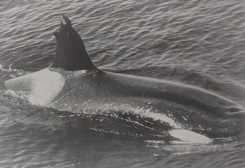
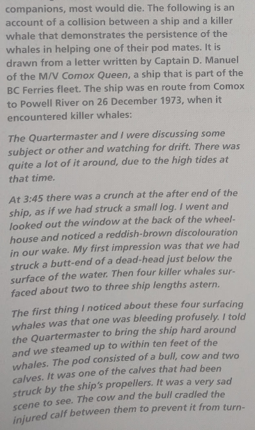
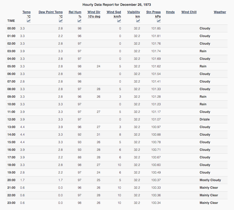
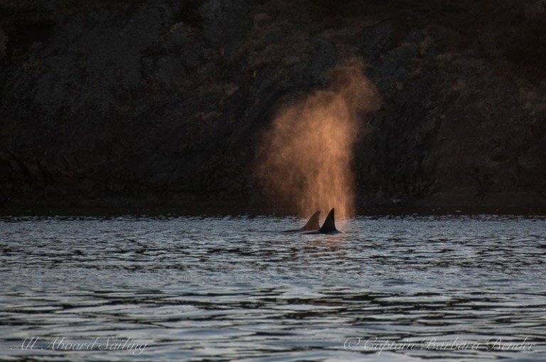
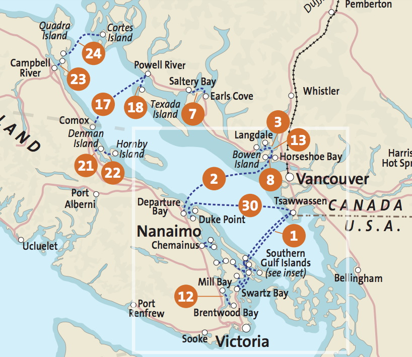
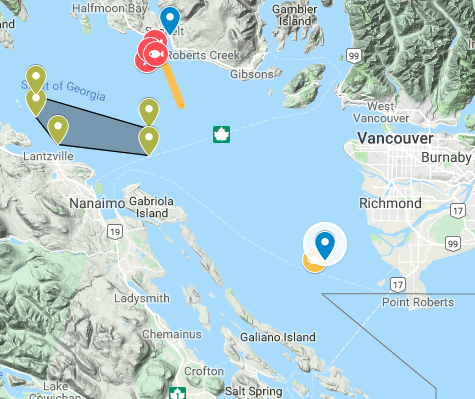
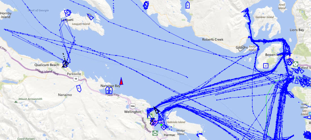
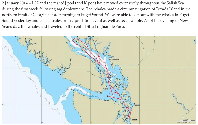
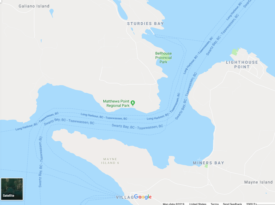
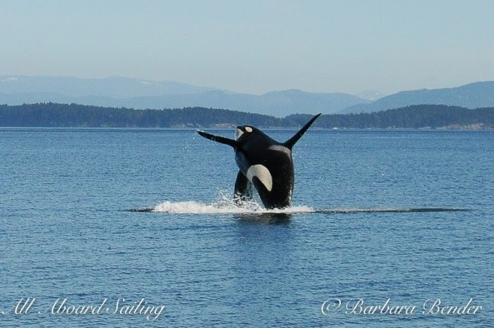
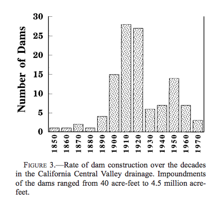
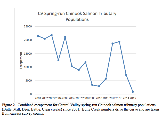
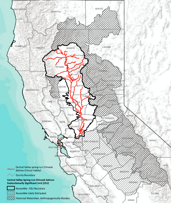
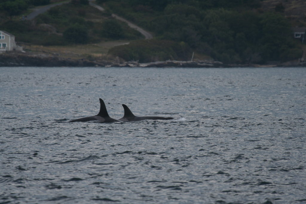
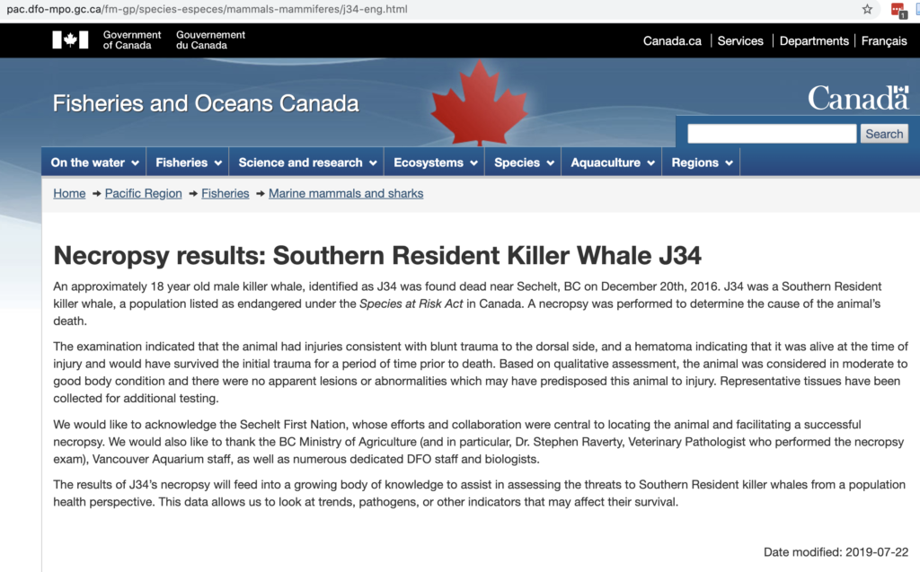
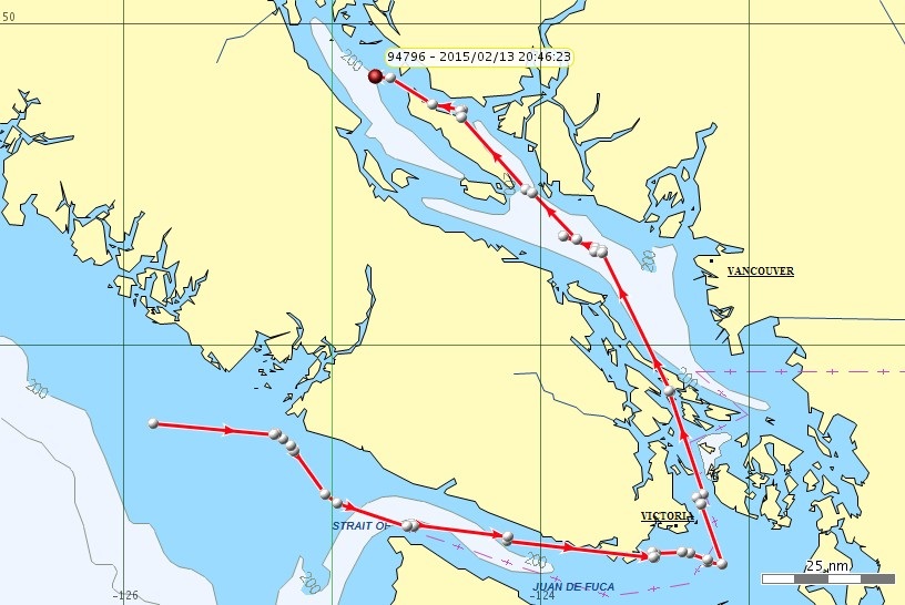
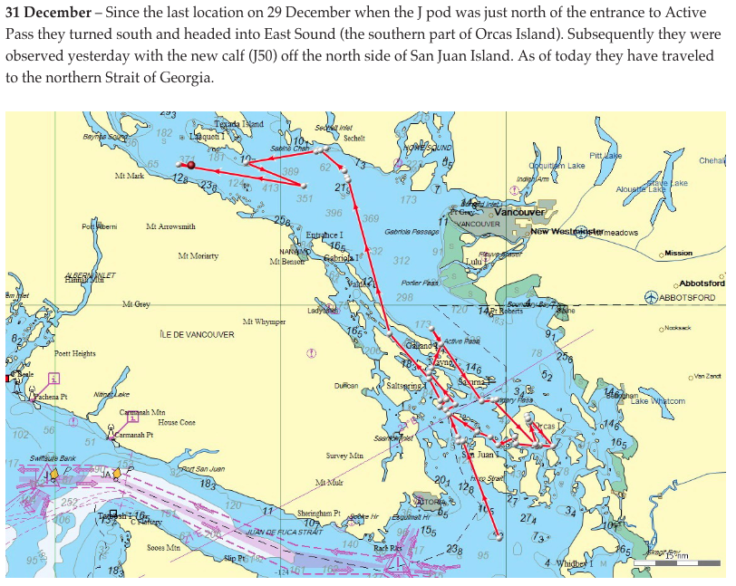
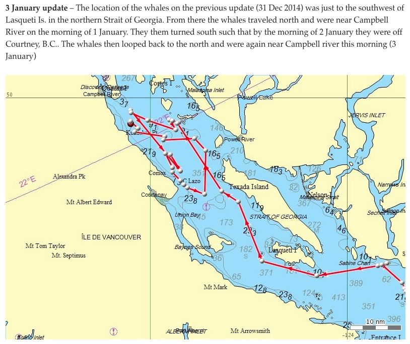
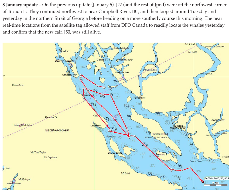
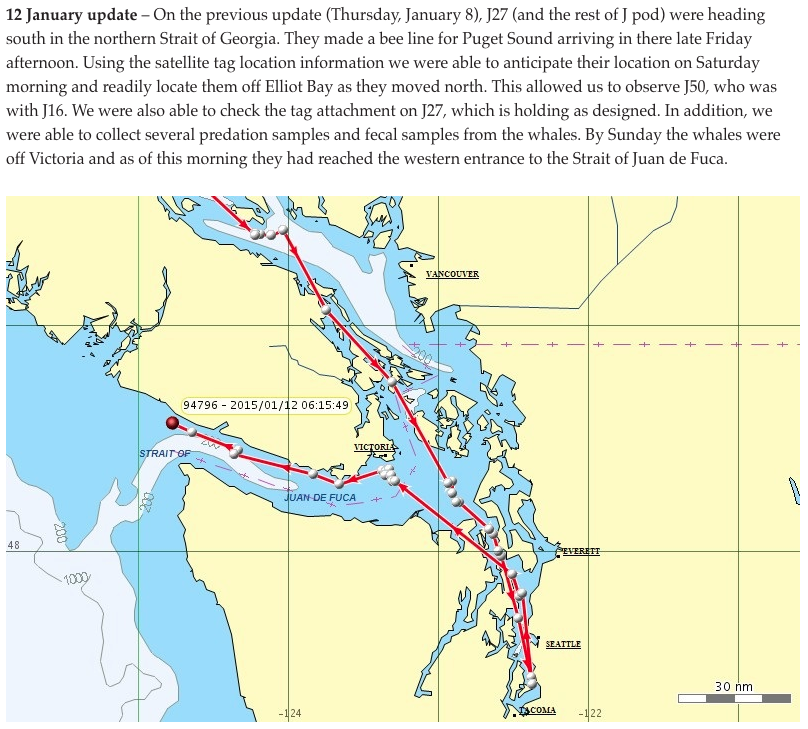
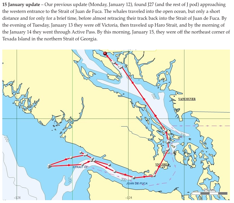
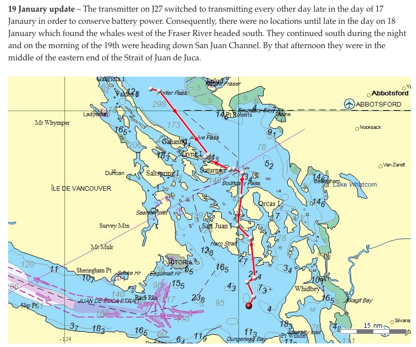

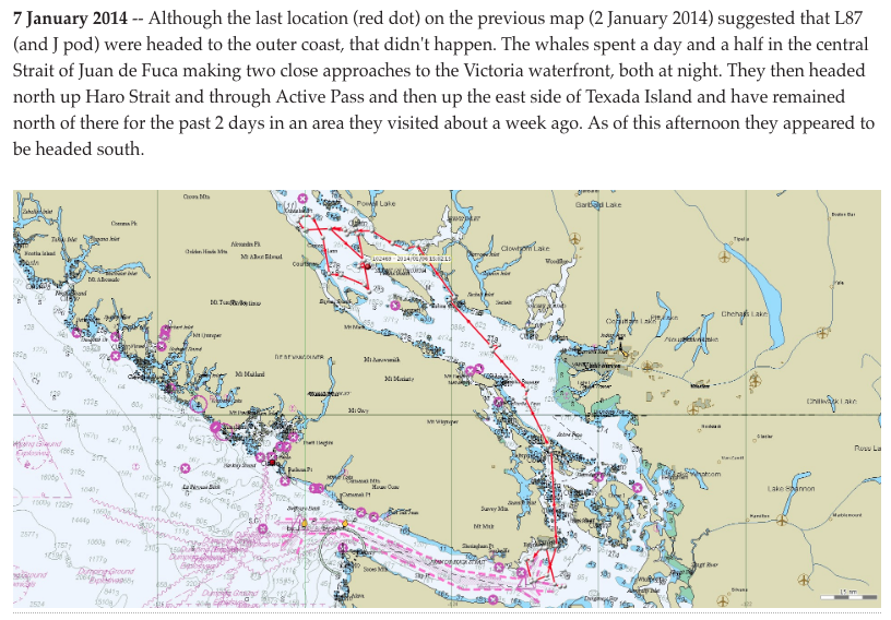
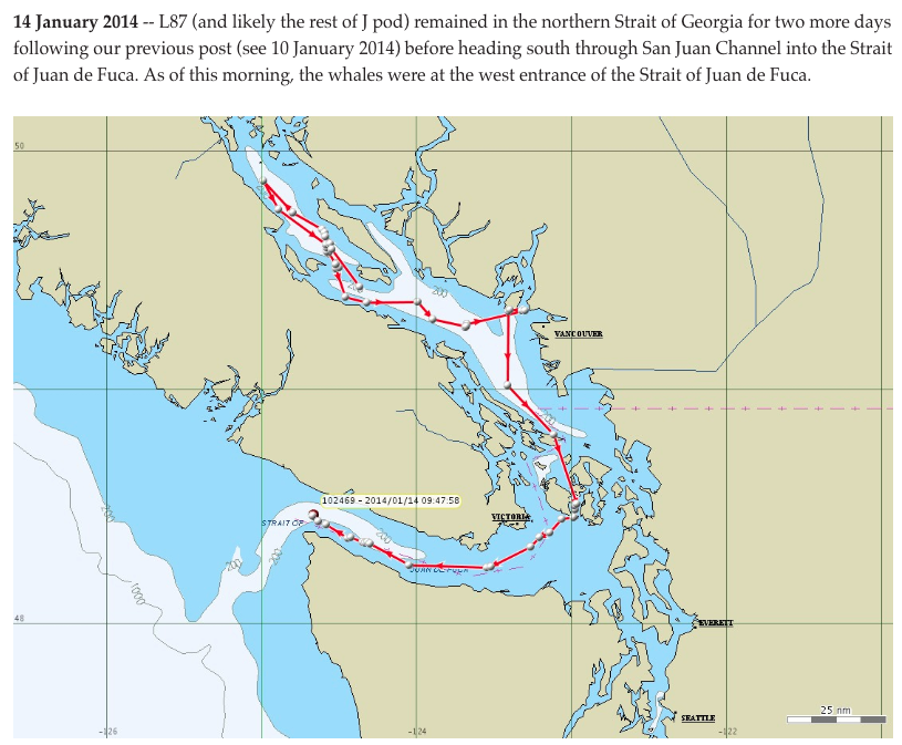
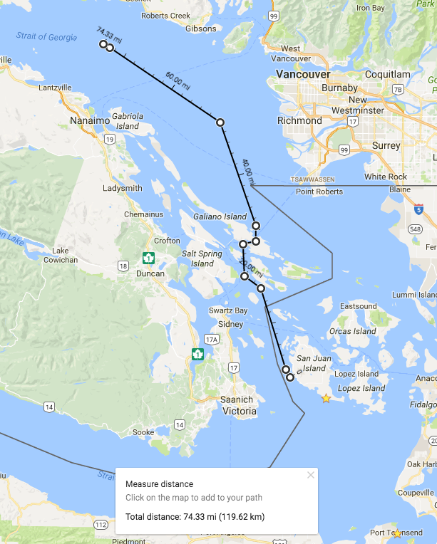
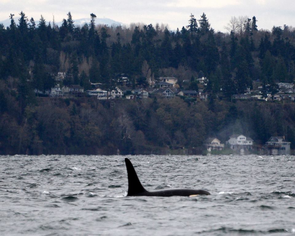
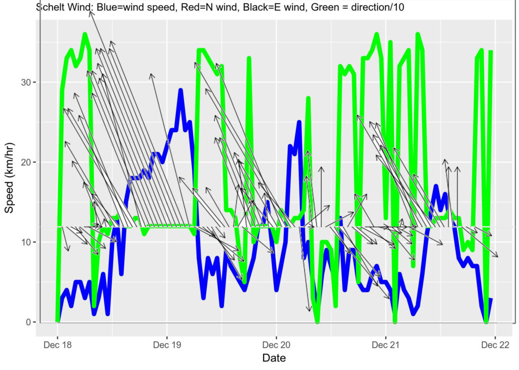
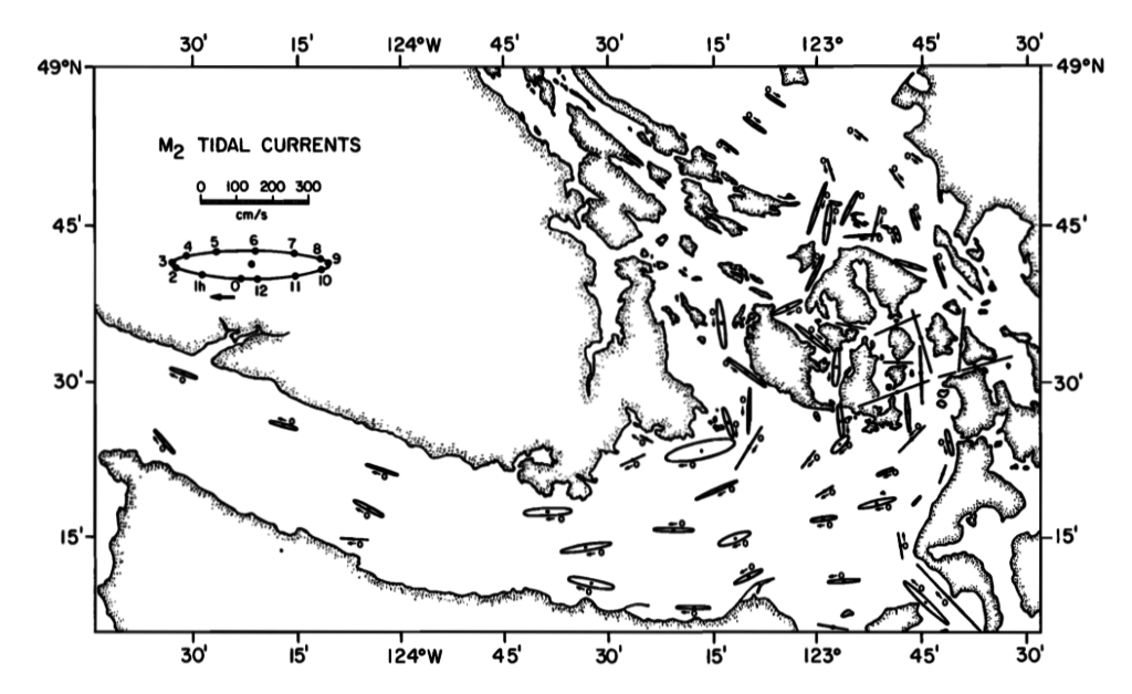
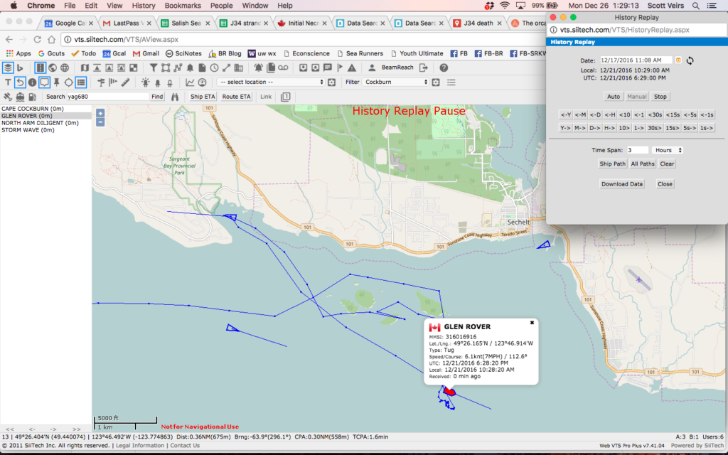
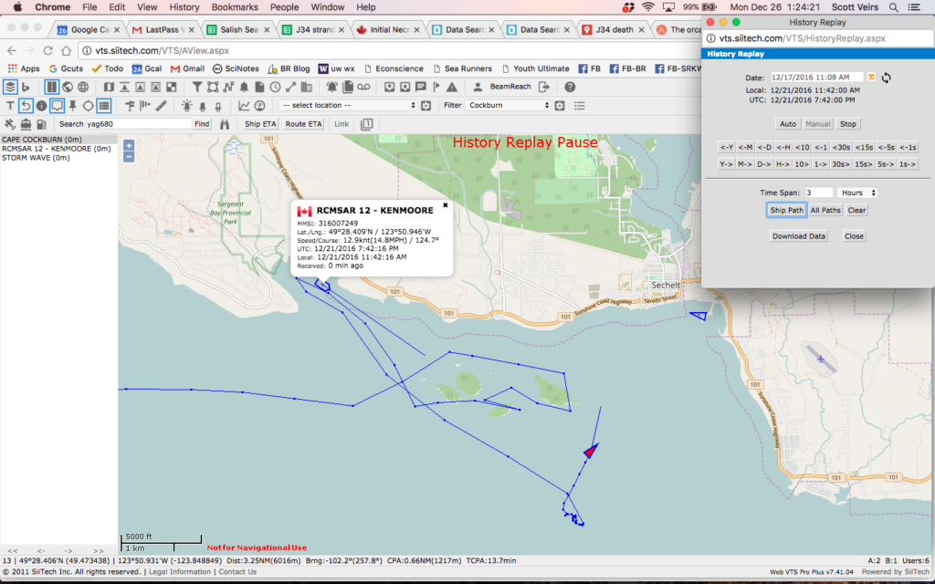
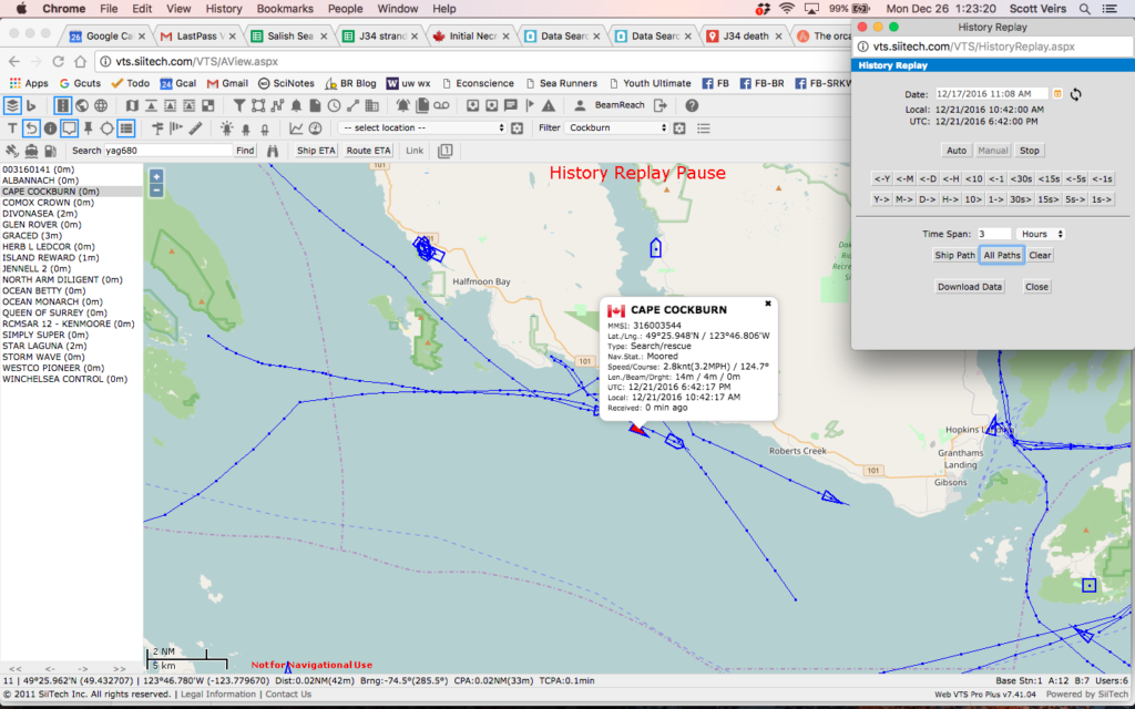
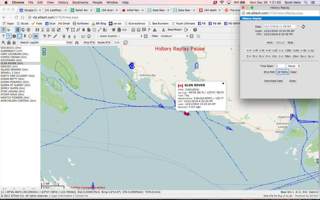
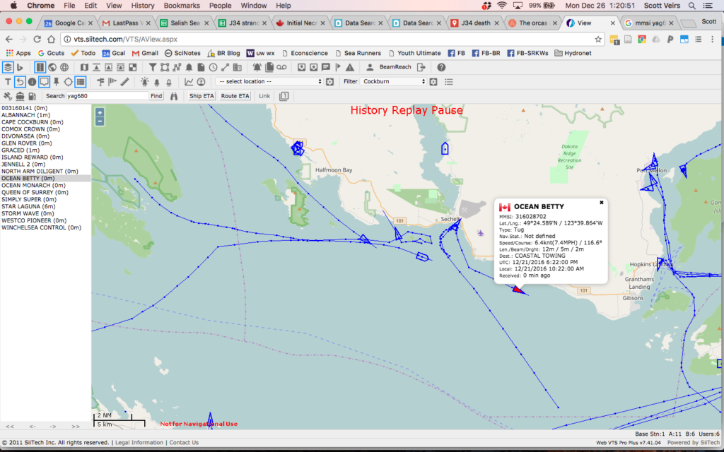
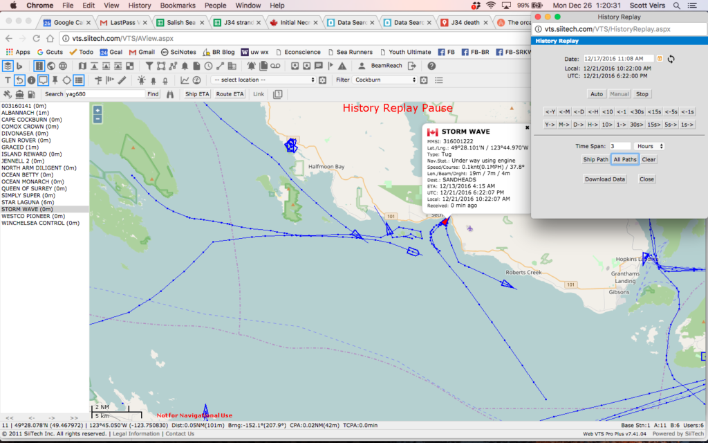
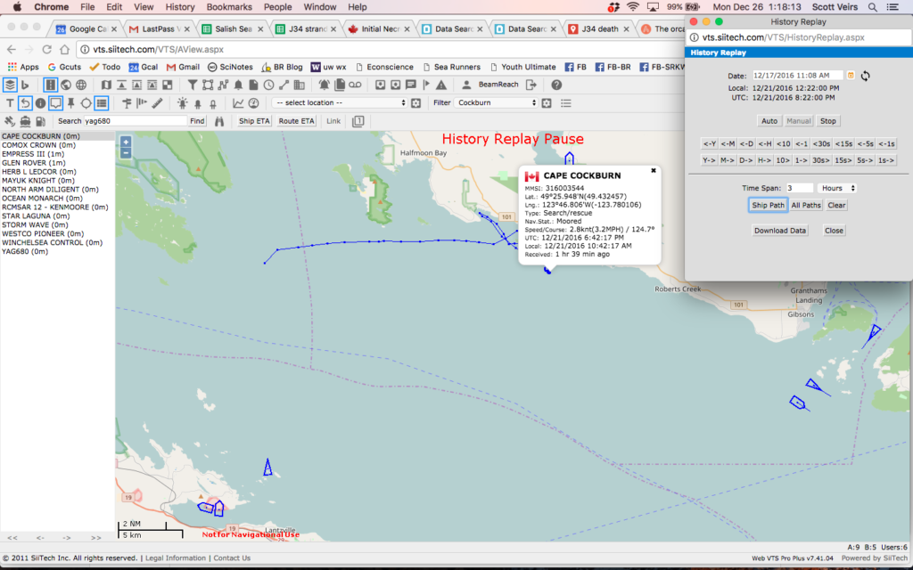
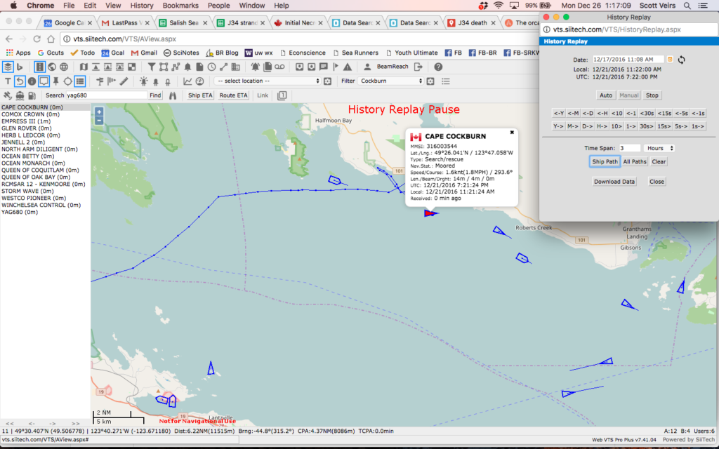
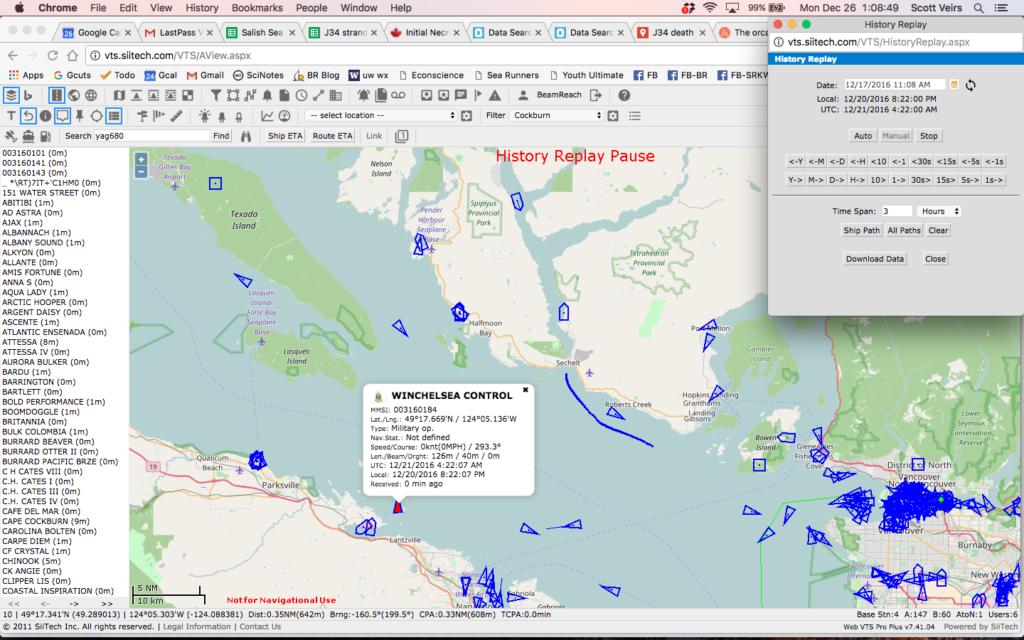
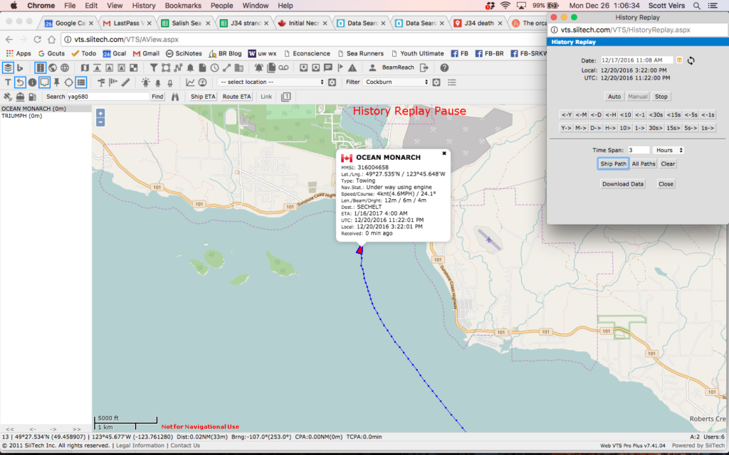
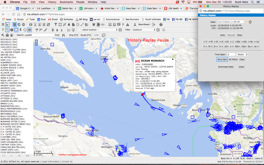
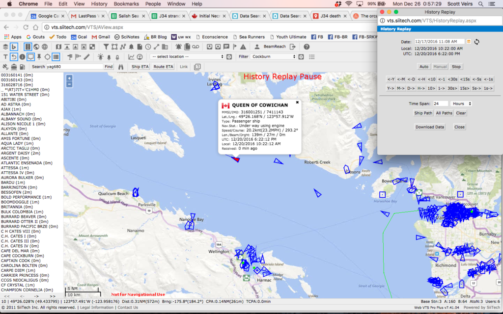
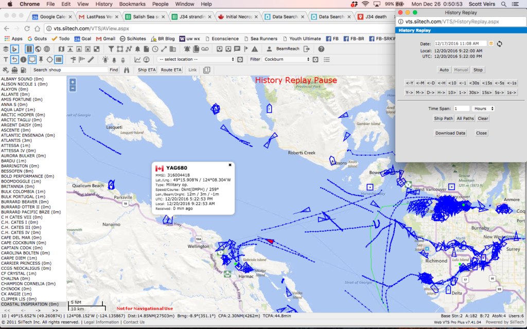

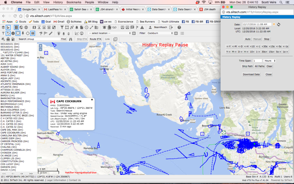
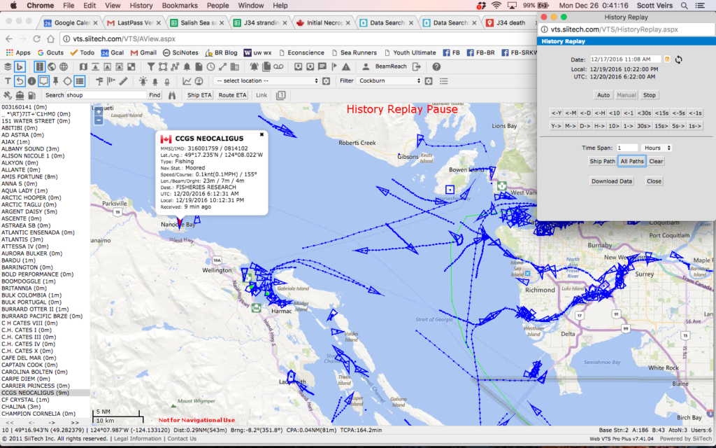
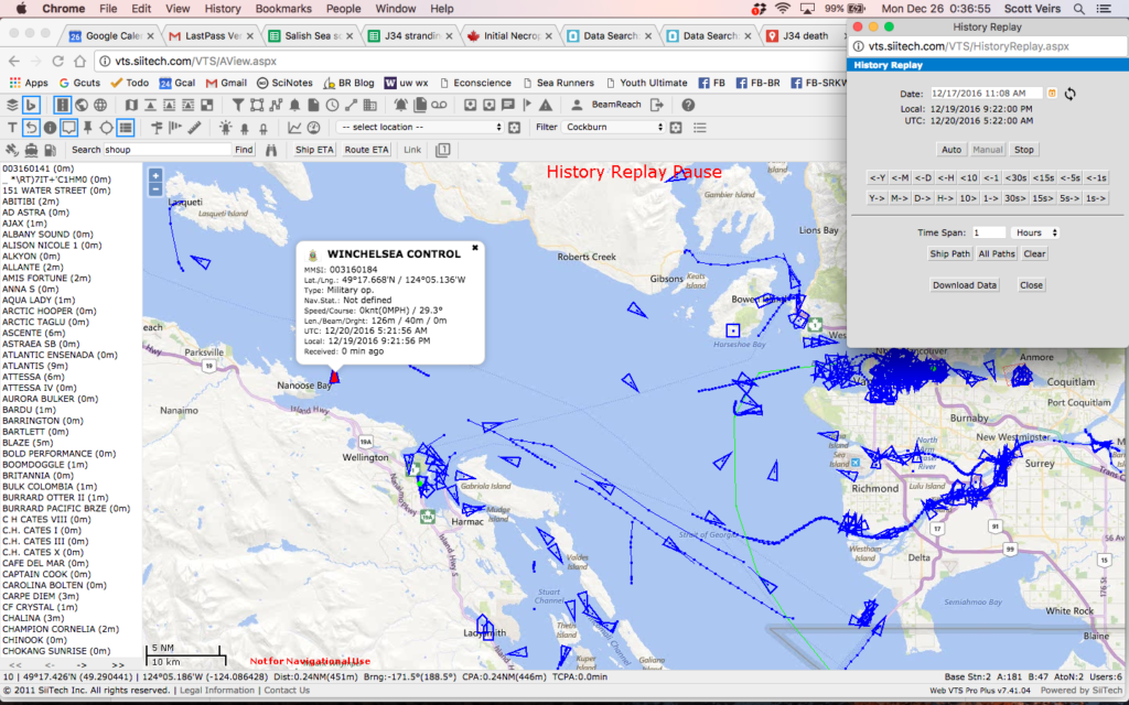
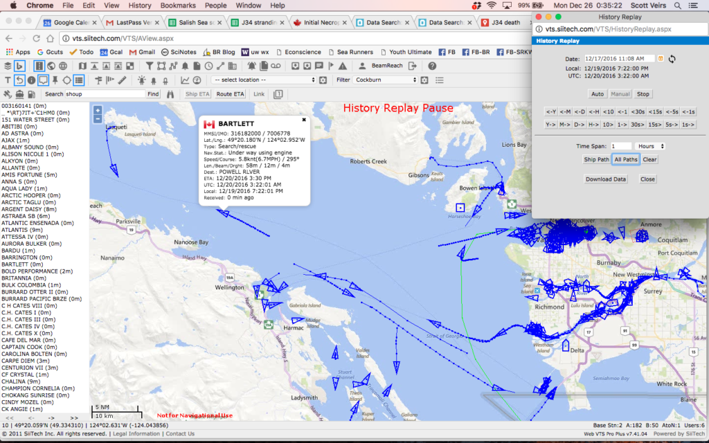
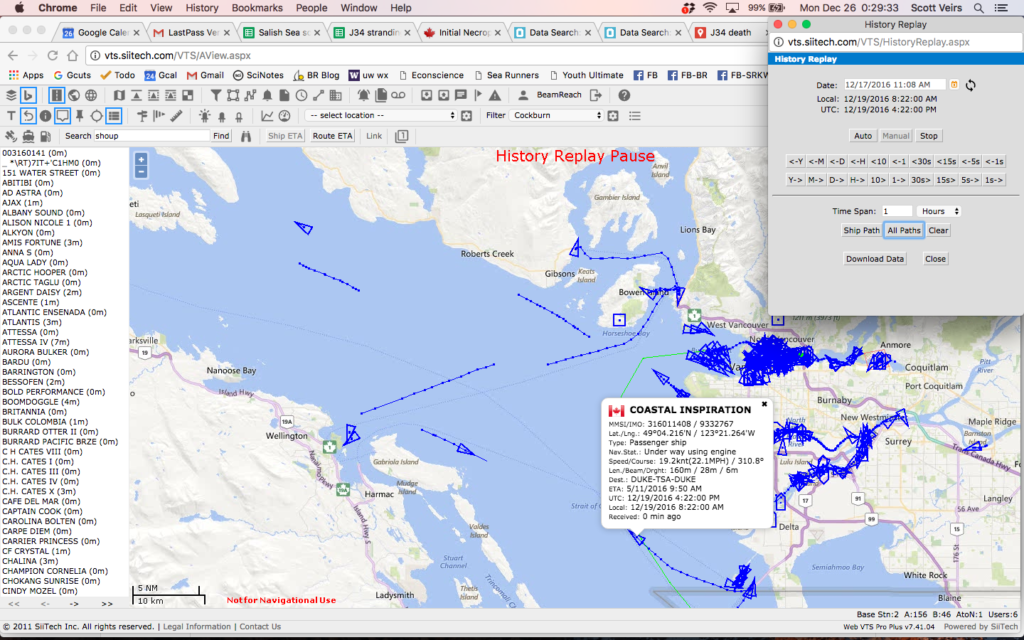
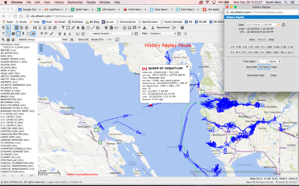
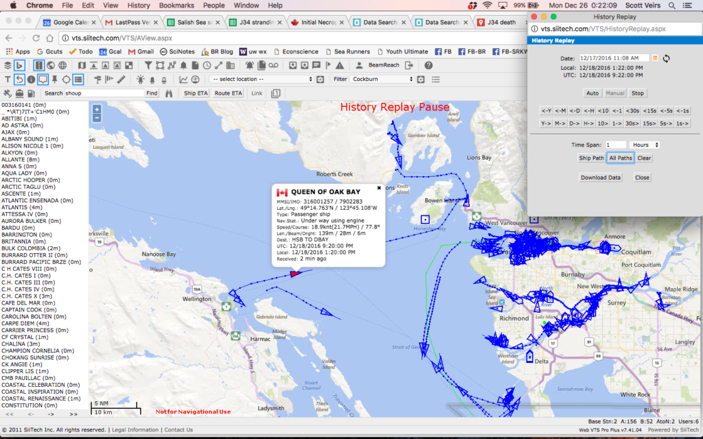
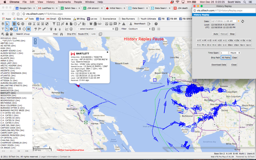
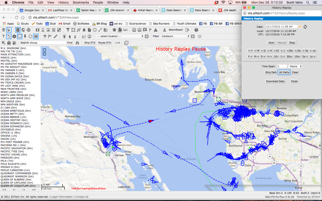
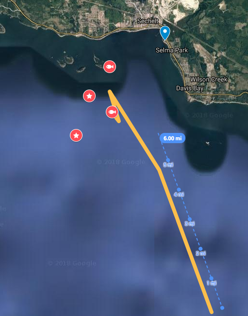
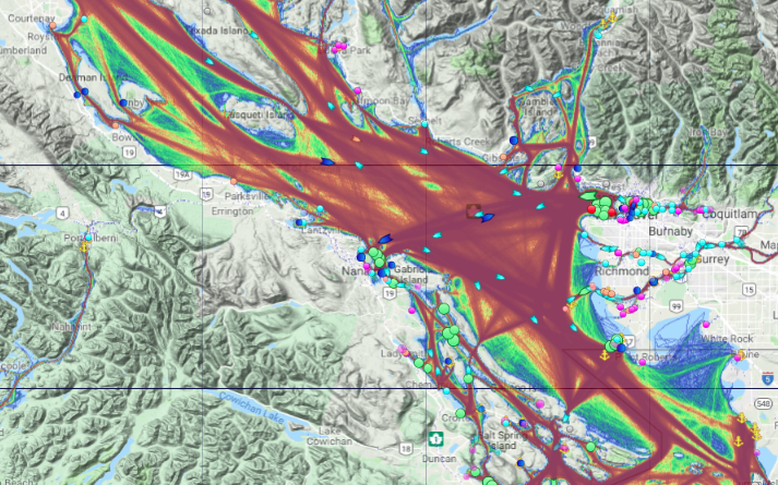
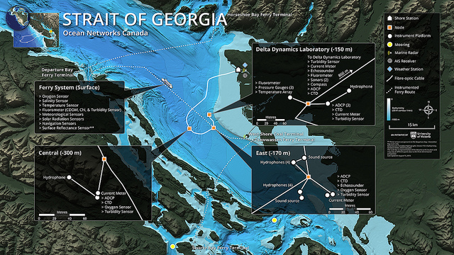
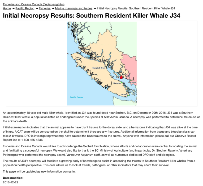
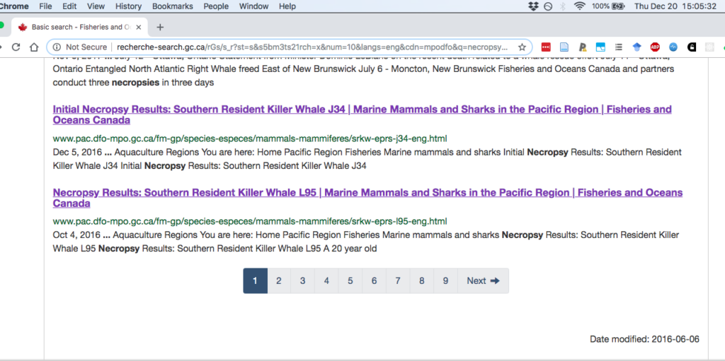
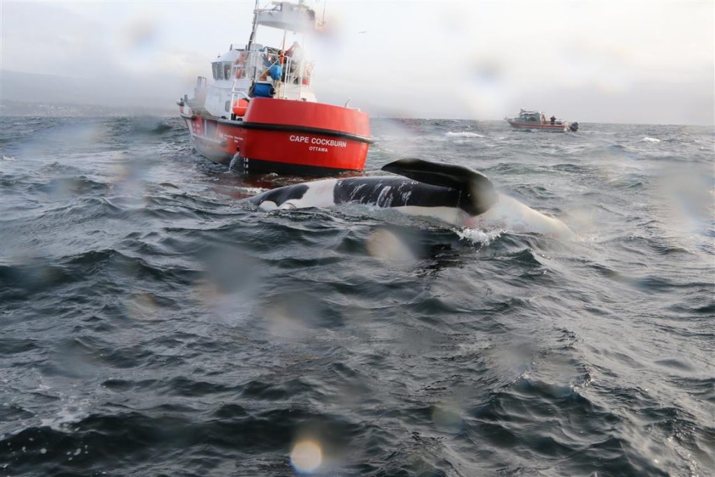
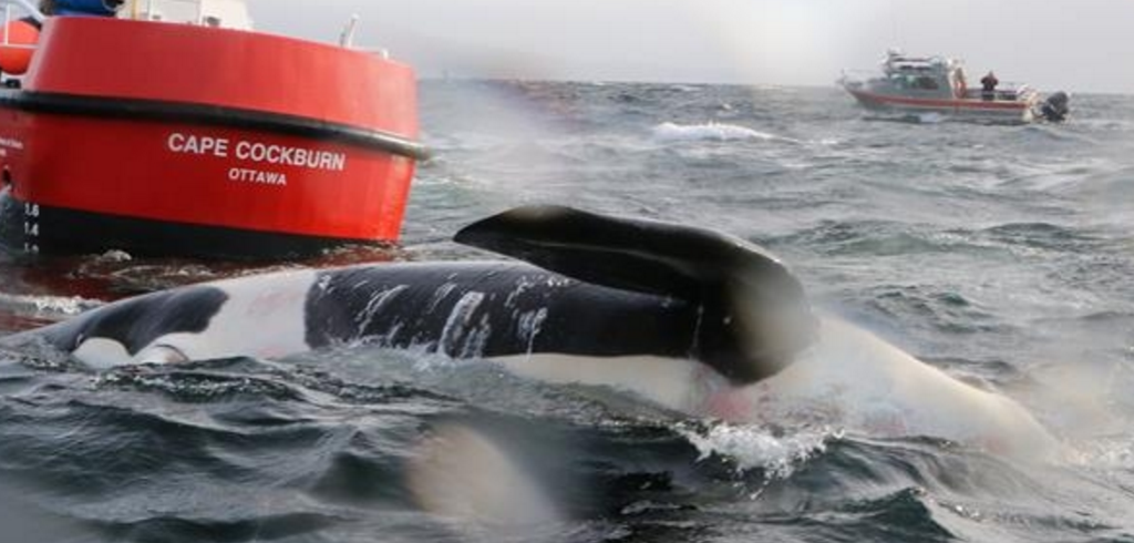
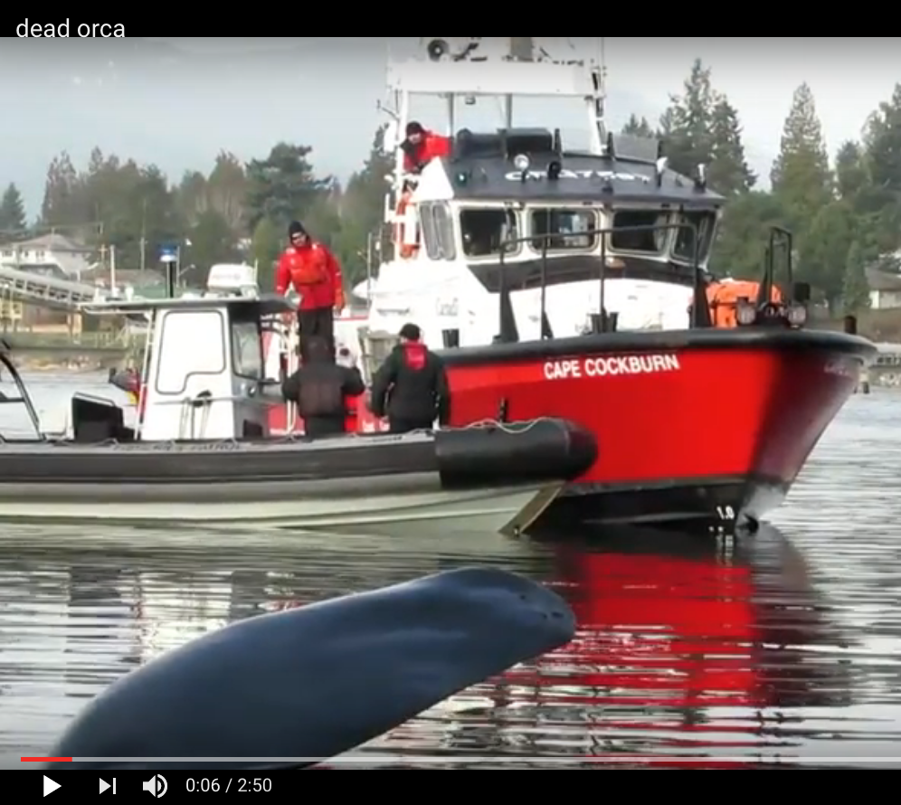
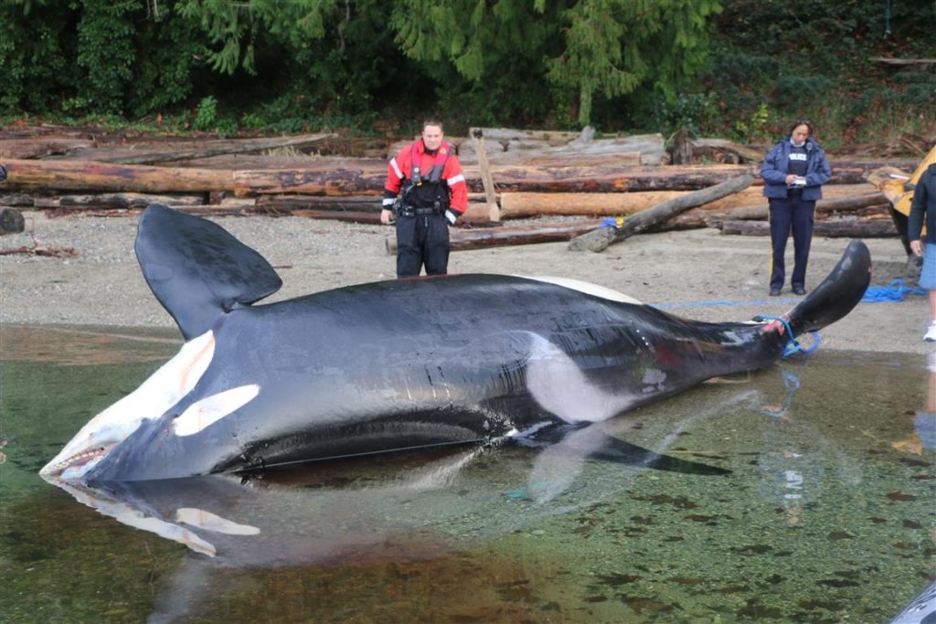
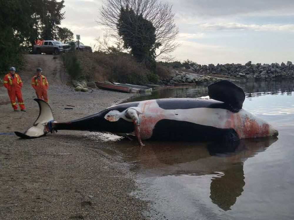
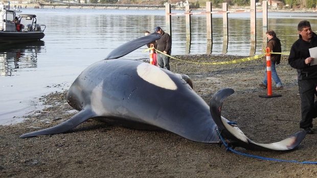

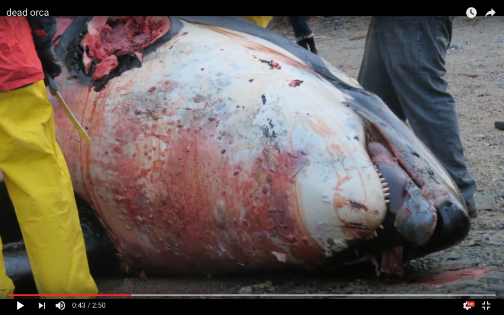
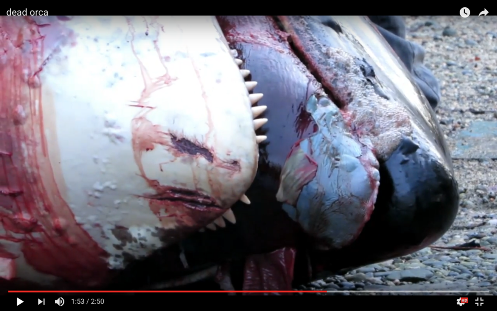
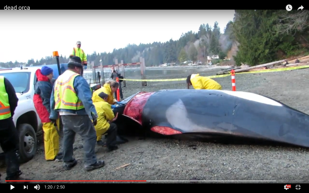
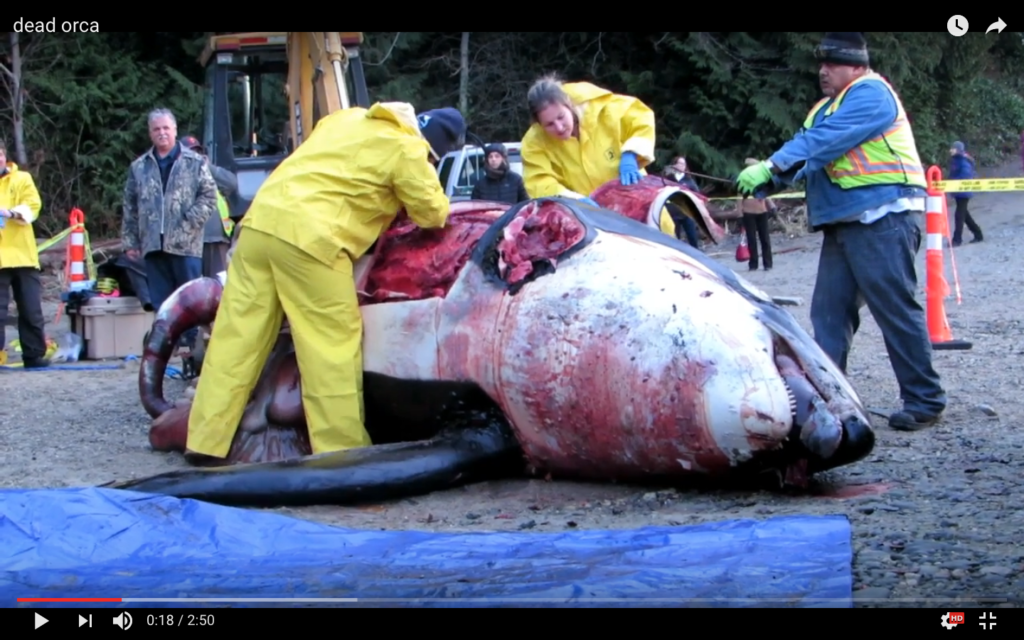
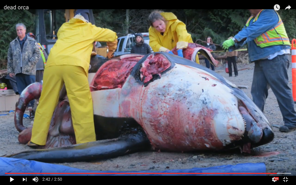
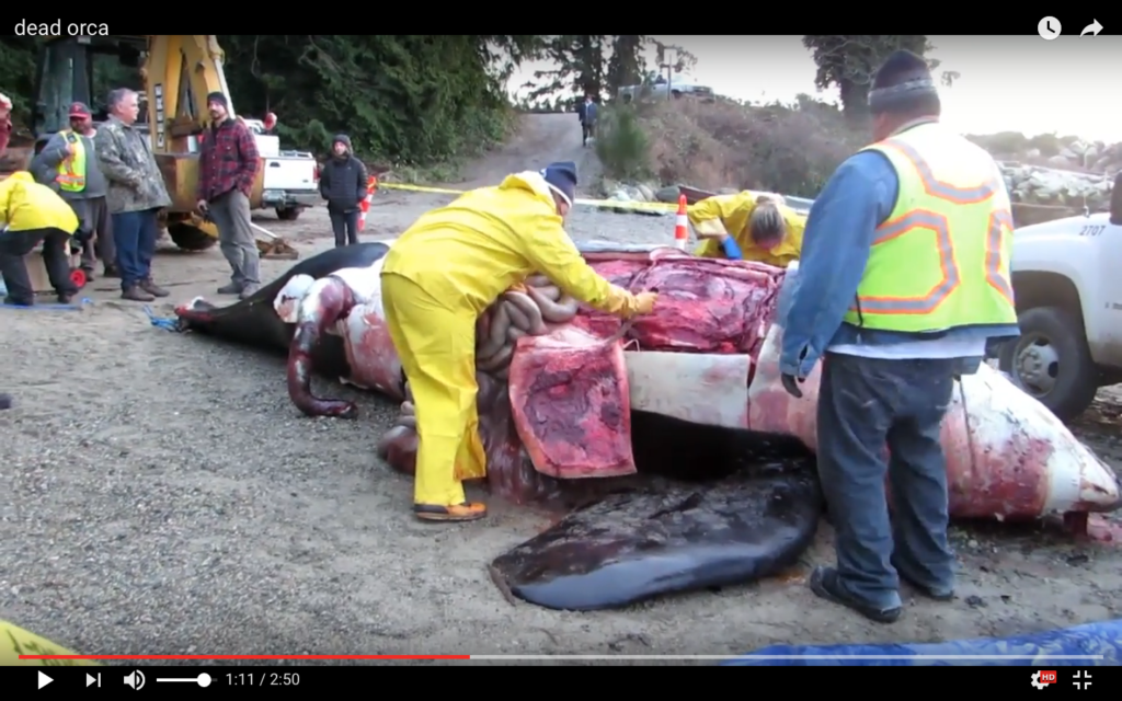
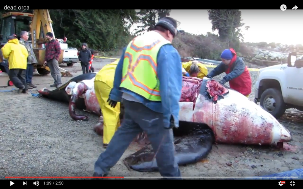
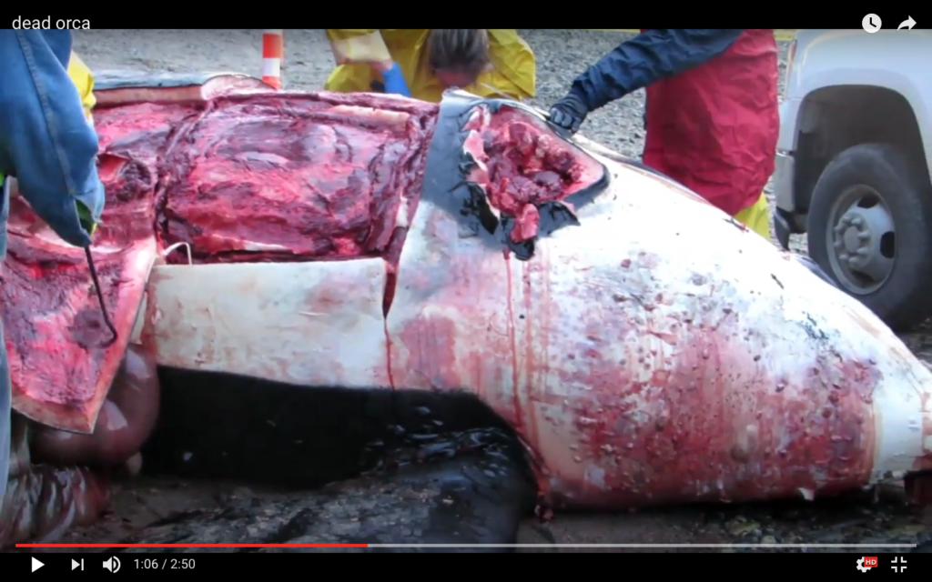
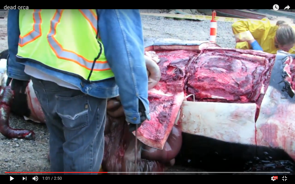
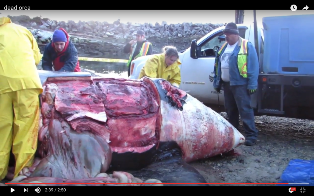

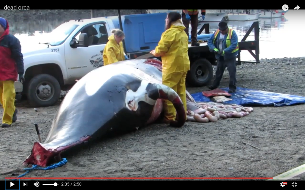
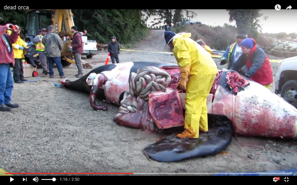
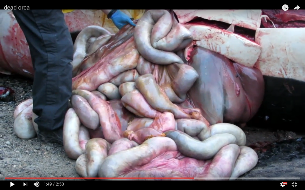
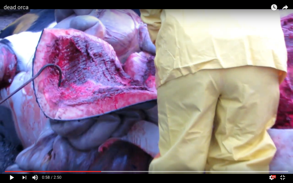
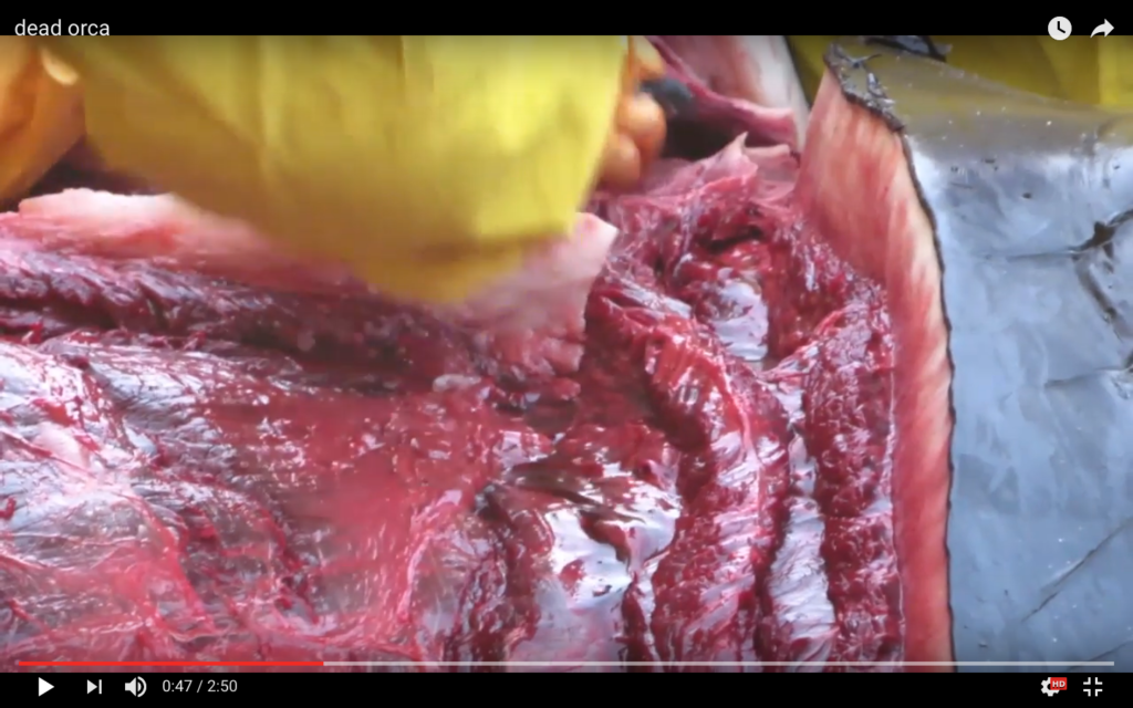
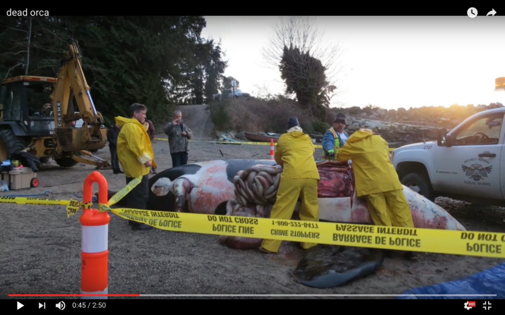
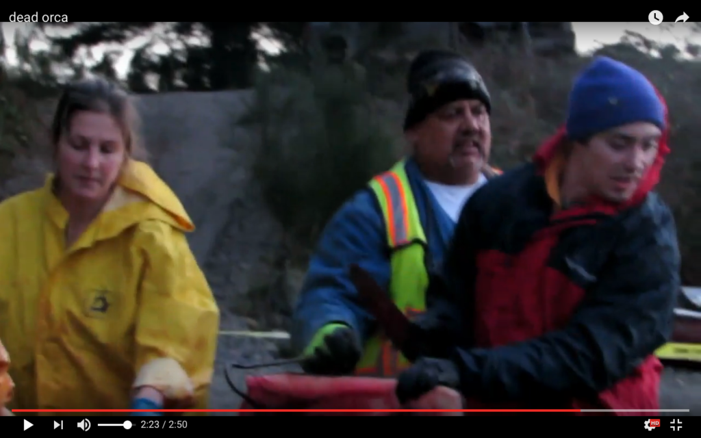
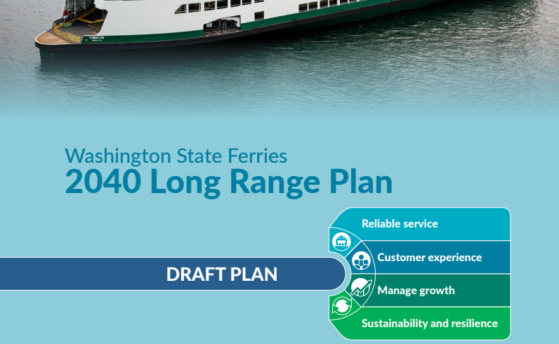
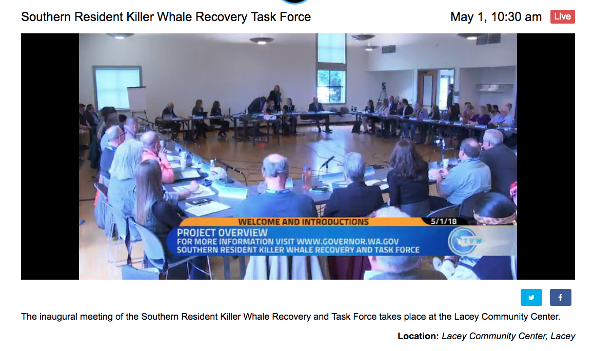
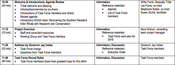
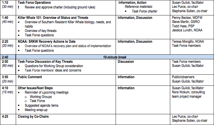

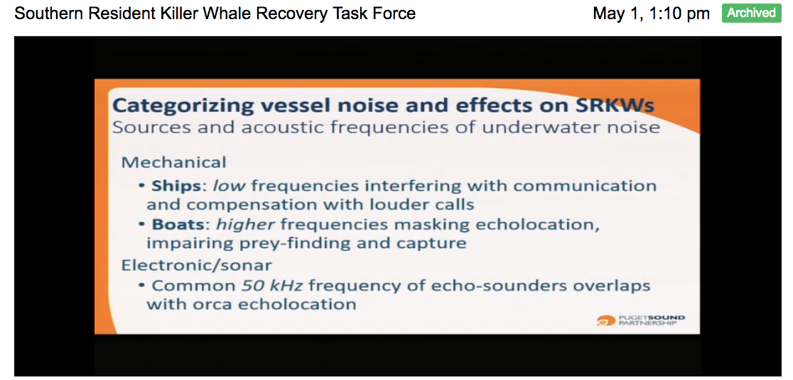

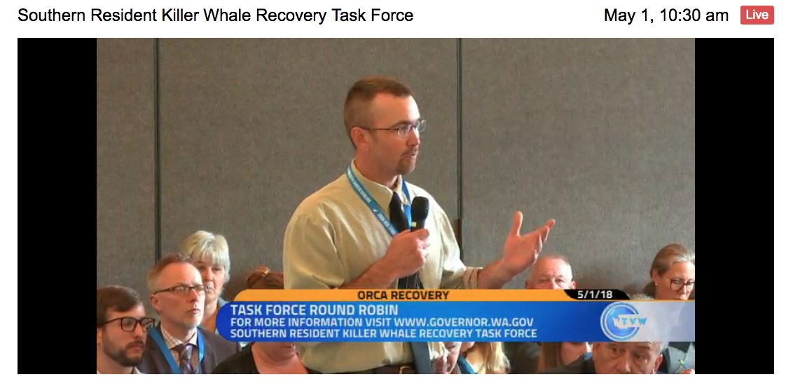
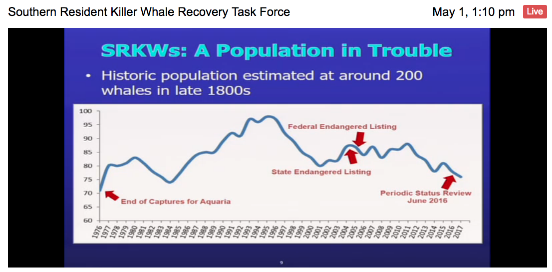
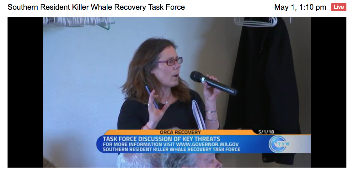
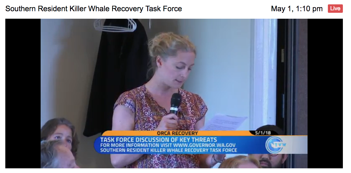

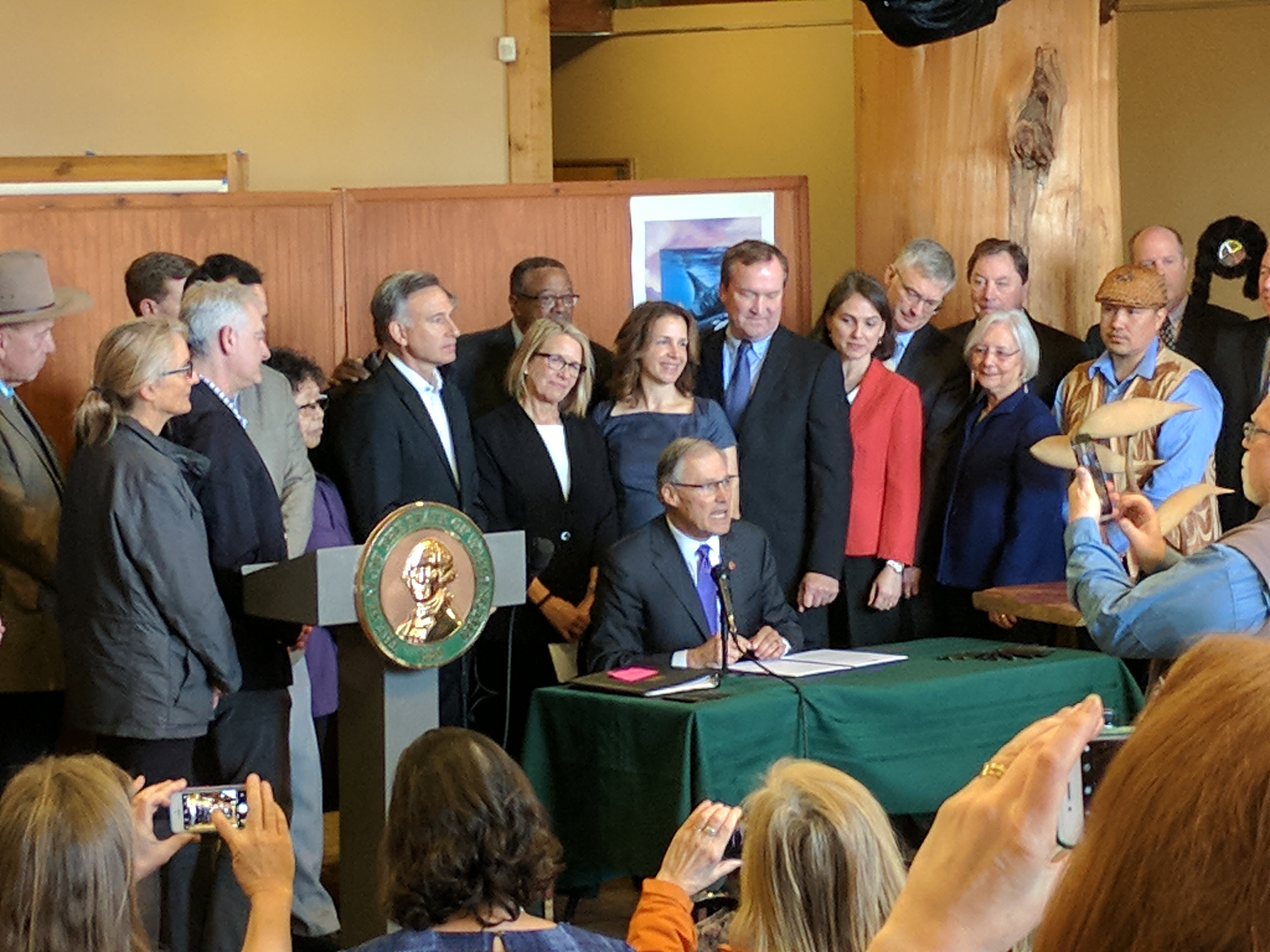
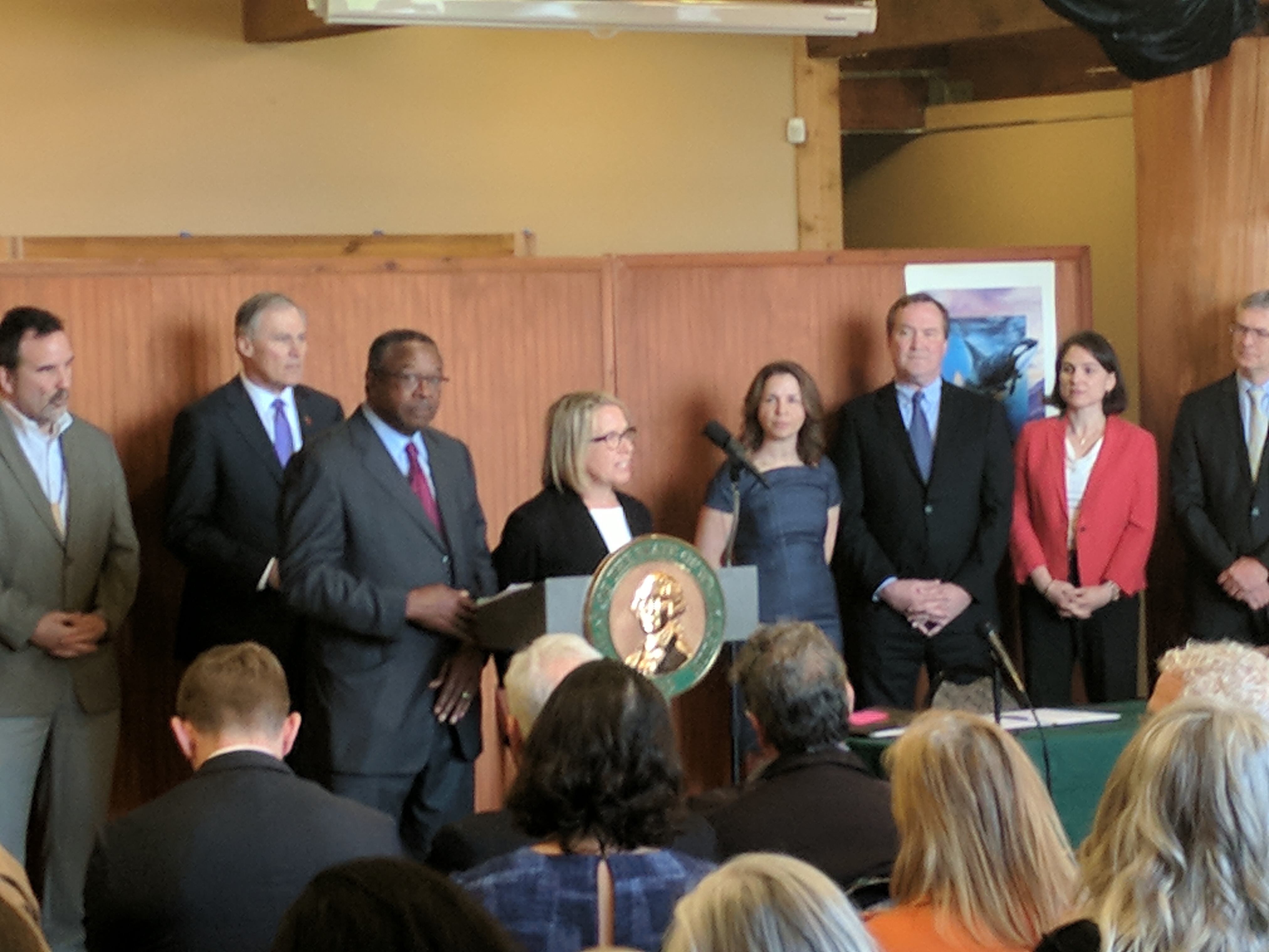
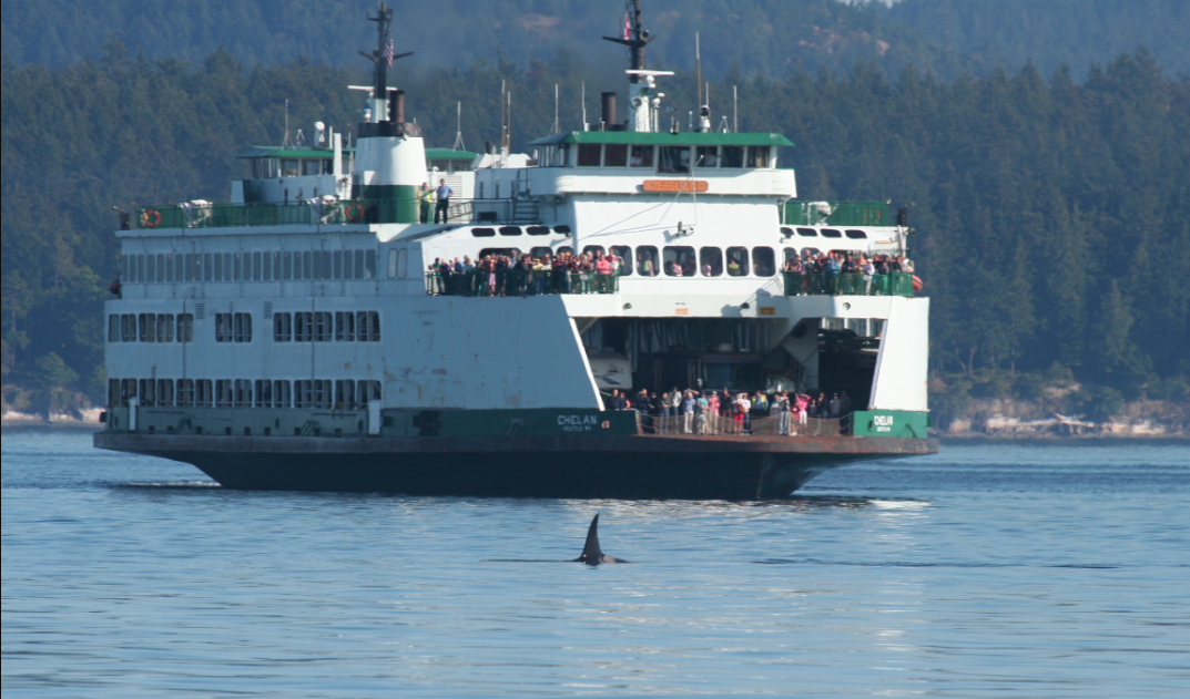
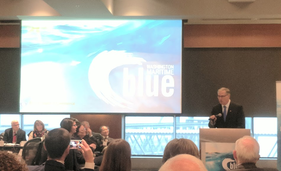
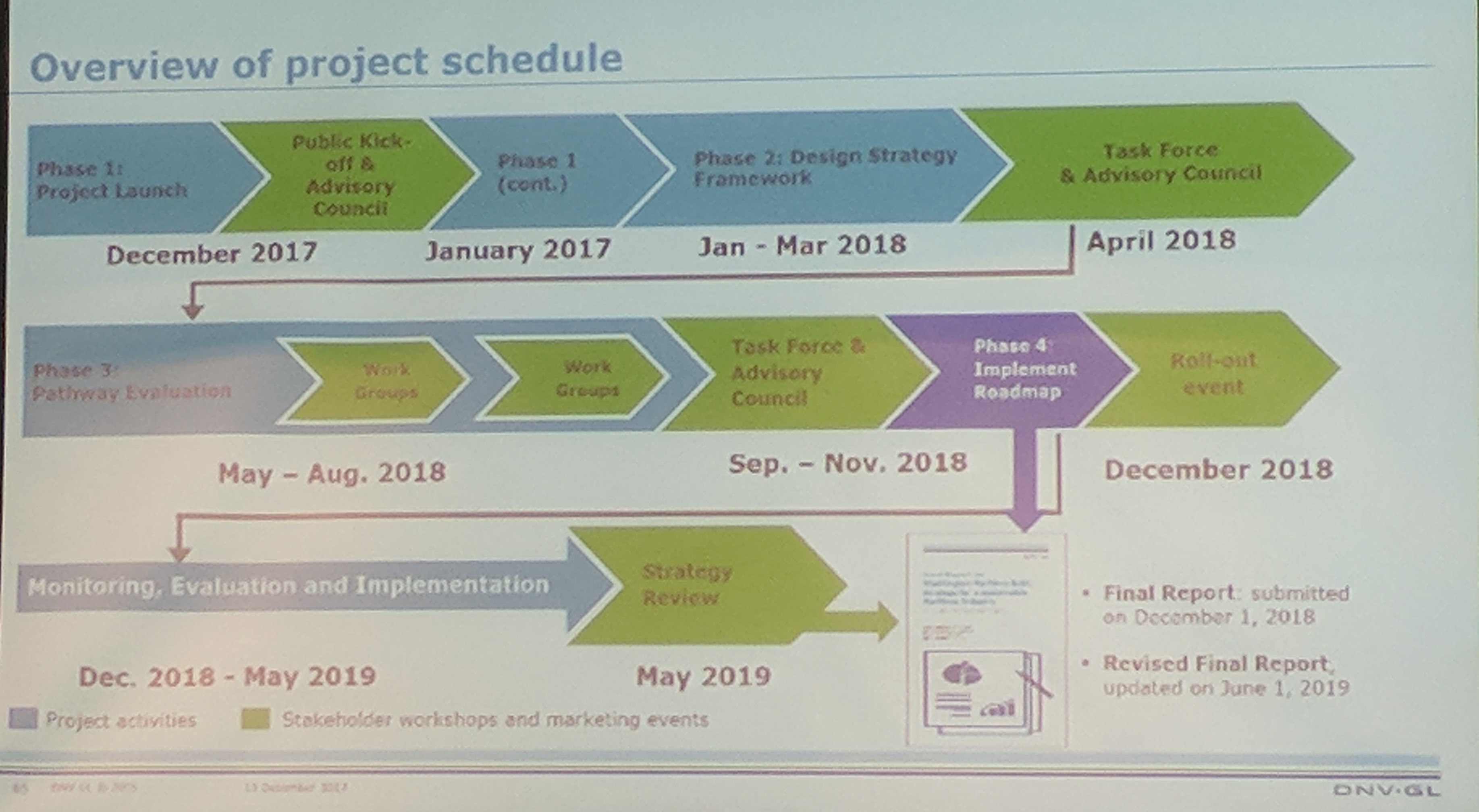
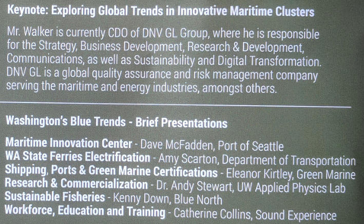
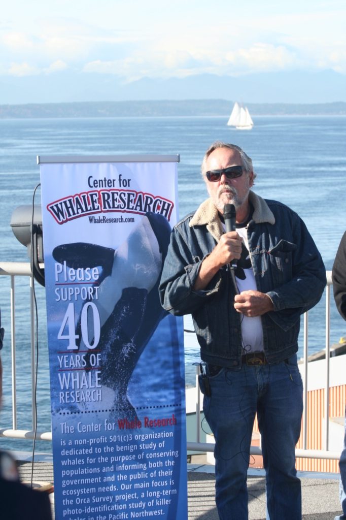
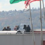
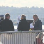
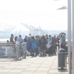
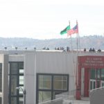
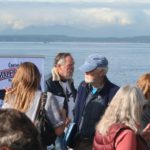
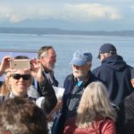
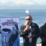
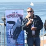
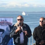
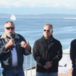
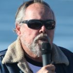


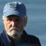
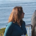
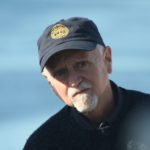

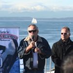
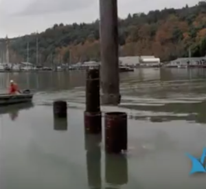


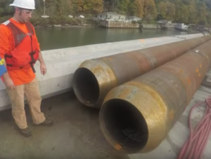
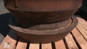
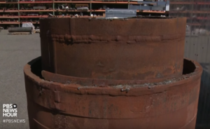
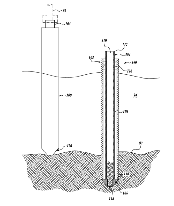
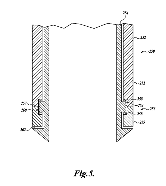
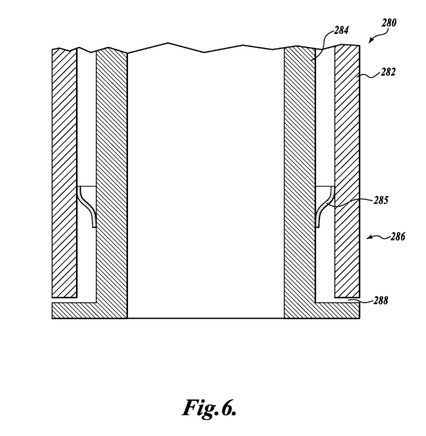
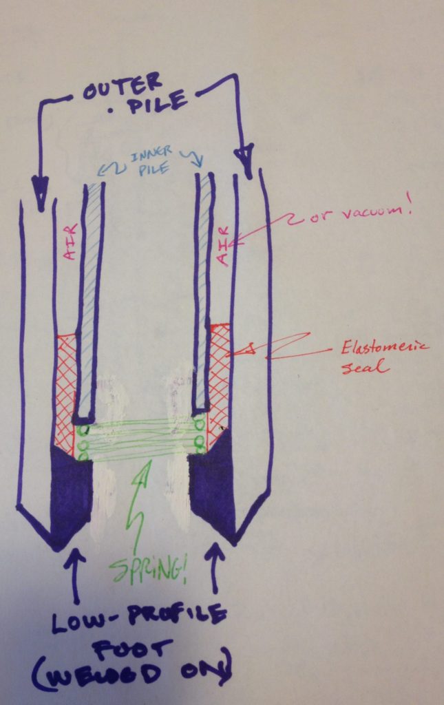


 Twitter
 LinkedIn
 Facebook