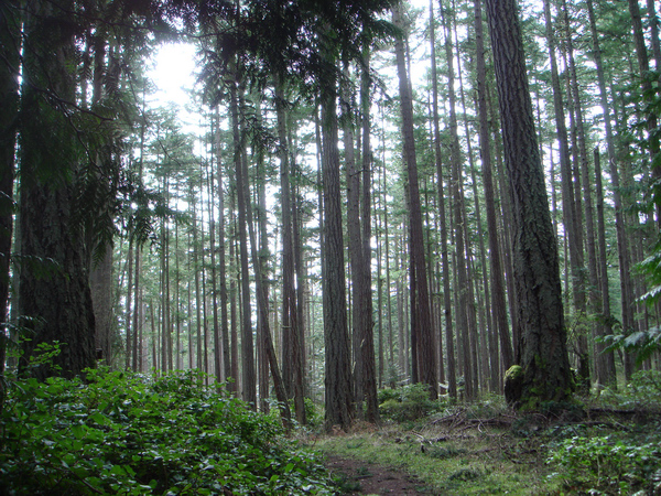
How did San Juan Island really look like 200 years ago?
Last Friday the S Pod had a case study discussion on sustainability. I chose an article entitled “Global Consequences of Land Use” by Foley et al, published in Science in November, 2005. The article pertains primarily to the effects of agricultural land use on land cover. One aspect I find intriguing is soil salinization, a phenomenon common in agricultural lands. Heavy irrigation of soil, coupled with removal of deep-rooted native vegetation, cause water table to rise near to soil surface. A disturbance such as heavy rainfall can then draw water levels to the root zone. When this water is evaporated from the soil surface, the salt is left behind, causing soil salinization, which quickly deteriorates soil quality.
Our Beam Reach instructor, Dr. Scott Veirs, mentioned that one common problem on San Juan Islands is the overwithdrawal of groundwater, causing salt water to seep into the aquifer. This led me to think more about the land and resource usage on San Juan Islands. In a conversation with Jason Gunter, owner of Discovery Sea Kayak, I found out that before English and American settlers arrived at San Juan Islands, the Native Americans practised controlled burning of open lands in order to better harvest bulbs. It has been speculated that at the time, many parts of San Juan Island were not forested. The theory is that controlled burning allowed slow-growing trees such as oak to mature. When controlled burning stopped, tall and faster-growing conifers such as Douglas fir out-competed the slower growing species by creating shades. These conifers propagated, which gradually brought about the landscape we see on San Juan Island today.
Jason has also mentioned that this change in land cover has caused the loss of a few species of birds. It would be very interesting to find out how land use and land cover have evolved for the past 200 years, and whether this has impacted the local nearshore or marine ecology in any way. Nonetheless, I think it is even more pertinent to study the current land and resource usage on San Juan Islands, in order to modify and adapt resource usage to ensure the continuous availability of these resources — such as potable water and fertile soil — in the future.
This week the S Pod, as we Spring 2012 Beam Reachers are now called, discussed at length about “sustainability science”. So, what is sustainability science? Each of us has a unique definition of what sustainability means to us, and many writers have proposed a variety of definitions.
My personal definition of sustainability has its foundation in the very meaning of the word “sustainable”. The word sustainable connotes, first, the “capability to be sustained”, and second, “using a resource such that the resource is not depleted or permanently damaged”.
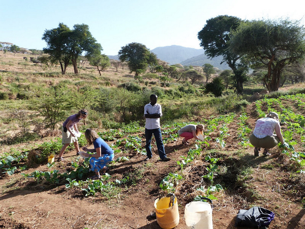
In implementing a “sustainable project”, it is important to make sure the project can be continued on a long-term basis. I recently visited a rural village in the Samburu region of Kenya, where NGOs have installed water filters for rainwater reservoirs. However, when I was there, the water filters were not functioning because the NGOs had failed to adequately educate the local community in how to properly use the filters. Therefore, one could say that this project is not sustained, and such a project is not sustainable if the local community does not get involved.
How does the above example translate to sustainability science, and in our case, environmental conservation? One of the most important element in sustainability is education. By imparting the knowledge and idea pertaining to one’s project to the local community, the local people could then become the engine of the project, and these knowledge, ideas and good practices could hopefully be passed down to the next generation and inspire students to become field-level experts.
Two days ago, Katie Fleming from REsources, an NGO based in Bellingham, WA, shared her experiences in community outreach. She implements a model which she calls “community-based social marketing”. This model markets an environmentally friendly idea or practice, such as to turn off the engine when the car is stopped for more than 30 seconds, by educating school children to influence their parents, giving small incentives, and by adding a “peer pressure” element”.
I feel that this is a wonderful practice in sustainability, in both aspects of ensuring the project is sustainable, and in promoting a more sustainable use of resources.
Moving on to the second definition of sustainability, which is the sustainable use of resources. The household definition of “sustainability” usually refers to the popular concept: to make use of renewable resources, and to reduce, reuse and recycle consumer products. One aspect of sustainability science could be to use a research method that is in line with the above practice, so that the research could be economically sustainable and have minimal impact on the environment.
Sustainability science in a larger scale would be to examine the current state of environment, and to encourage essential economic practices such as agriculture and transport, to move towards the sustainable use of our shared natural resources.
Our Beam Reach instructor, Dr. Robin Kodner shared with us her personal definition of sustainability during our round-table discussion. One of Dr. Kodner’s current research project is to measure the level of Domoic Acid, a neurotoxin produced by the diatoms Pseudo-nitzschia, in nearshore waters. Her hypothesis links higher levels of Domoic Acid in the water with altered water temperature or nutrients leached from agricultural lands.
Dr. Kodner’s definition of sustainability science is: using natural science methods to study the social and environmental interactions and changes, hence providing the data as a basis of better management and policy. And also, to come up with innovative solutions.
In Kenya, our class did a small insect abundance and variety survey on subsistence farms. Our investigation was brief, but we compared and critically assessed the condition of the two farms. The overarching goal of such a survey was to reduce pesticide use by relying on native species to reduce herbivory on crops. One method is to have weedy margins to agricultural plots. Reducing pesticide use reduces the amount of toxin that could be leached into streams or groundwater, which helps to ensure the sustainability of local water resources.
Insect Abundance and Variation Survey in Kenya, 2012
I am really glad that my experiences in Kenya have enabled me to contribute ideas in this class. My current research direction is to find out what aspects of orca conservation might human interest come into conflict against. I look forward to learning more about the Salish Sea and my beautiful classroom — San Juan Islands!
Live blog from the second workshop on “Evaluating the Effects of Salmon Fisheries on Southern Resident Killer Whales” began today (3/13/2012) in Vancouver, B.C. During this second step in a process NOAA initiated to manage chinook salmon with attention to southern resident recovery, a U.S.-Canada science panel will revisit some of the questions posed during and after the first workshop, including: population status; feeding habits; fisheries that may affect prey availability; relationship between Chinook abundance and population dynamics; Chinook needs, abundance, reductions, and food energy available. Specific goals are to discuss changes to the population modeling (FRAM, Baysian posterior estimate) and review new data on winter food sources and availability.
Most presentations include links to the slides (PDF or PPT) archived on the workshop web site. Select presentations also include a link to the audio recording of the presentation.
Day 1 (3/13/2012)
8:45 Ray Hilborn reviews science panel impressions from first workshop
His presentation summarized the types of information requests that will be addressed over the 2.5 day workshop —
– Explore the different hypotheses of why the SRKW population is so small
– How does the density of SRKW compare to the densities of KW in other areas?
– What are the legacy effects of removals for the aquaria trade?
– What else is eating Chinook and how much are they eating?
Ways that indigenous knowledge systems could increase awareness of the contribution these knowledge systems can make to natural resources management.
There are 5 different names for eulachon (including a general term and names for successive runs, indicating to fish biologists that there are 4 runs of returning adult eulachon).
In Tlingit, there are 3 names for 3 artistic depictions of killer whales (‘sit, or ‘kit) which may represent a “point of convergence” of indigenous knowledge and scientific recognition of three regional ecotypes: offshore, transient, and resident.
Is the population declining?
While SRKW population has declined in some years historically, estimates of λ are overwhelmingly positive (mean λ of 1.023)
Remember:
• Lambda (λ) quantifies the long term time- invariant, deterministic growth rate of a population at equilibrium
– “long term†= on scale of decades
– Replacement of females by females
– *Different than regression of population size!
– Environmental and demographic stochasticity – Population age and sex structure
NOTE: juvenile survival is most important [with implications for the death of L-112 who fell in the age 2-10 year-old age class in the model]
How have actual growth rates changed?
Why isn’t the population increasing more quickly?
Possibly because there is a male bias in the southern residents…
All pods have positive growth rates, and K / L pod’s expected growth rates appear to have increased recently
Sex ratio at birth
— 45% of births since are female (44/96 v 76/140)
— NOT a statistically significant difference
Males, males, males
Reproductive and younger animals (< 20)
Stochastic birth and deaths
The male bias in the wild southern resident population may be due in part to a sex bias in the historical captures.
Why are there more males?
1. Compensation for historic removals? (male biased harvest)
2. Compensation for lower survival rate (males v females)?
3. Interaction with contaminants?
4. Trends in age of male or female SRKW?
Moose: as mean male age drops -> fewer males
BUT mean male age in SRKW has gotten younger
5. Older males more likely to father male offspring?
– White tailed deer, old SRKW males father lots of offspring
6. Density dependent response to slow down population growth?
– Generally opposite of what’s been observed for other long-term studies of mammals (red deer, sheep, other ungulates)
How do southern and northern resident models (posterior distributions) differ?
SRKWs have lower fecundity — For females of a given age (23), NRKW fecundity is on average 35% higher
Mortality rates are different (not comparable as reported in 1st workshop)
NRKW are about 130% higher (not 200% as reported in 1st workshop)
Apply mixed effects models to examine variability among clans / pods / matrilines
Correlated population trends in SRKW and NRKW
Updated comparison of density dependence / covariates, with NRKW and SRKW
“Age is the major driver of fecundity, with co-variates like salmon being secondary.”
Models with density dependence (esp females) do better than salmon only models
 What drives fecundity and survival? — Prey? Density dependence? Both?
SRKW and NRKW populations are correlated (e.g. drops in the 1990s are likely due to environment (and not age structure of SRKW)
Summary slide
1. SRKW have smaller λ than NRKW
–  Lower fecundity
–  Lower survival
–  K/L pod have skewed sex ratio (< 40% female in recent yrs
–  Fewer female births
2. Estimating random effect deviations for SRKW is difficult
– Regional (N/S) difference is better predictor
3. Fecundity: SRKW and NRKW have a similar response (+ with + salmon) – Suggests salmon difference isn’t responsible for smaller growth of SRKW4. Survival: density dependence (total females) receives most support
–  DD effect is weak in SRKW, less than the effect of increasing CTC index
–  DD effect is stronger in NRKW & smaller than salmon effect
–  DD effect too small to explain the lower λ (or survival) for SRKW
5. Support for “Moran’s effect†(correlated dynamics between NRKW and SRKW), synchrony a result of environment because dispersal=0
– Populations correlated, drops in the 1990s likely due to environment (and not age structure of SRKW)
Whales per square kilometer in resident populations
Perhaps the SRKW population has always been small?
How does the density of SRKW compare to the densities of KW in other areas – NRKW, Alaska, other?
Peak size reconstructed from life-tables = 96 (in 1967); +5 captures from 1962-1966; = 101 whales if all captures had livedWiles (2004) obtained a similar number (117) by adding all captures to population size in 1971
Note that the number of whales per 1000 km^2 varies and is often driven by productivity of habitats. SRKWs are about 0.9 whales/km^2, vs 1.7 for NRKWs, 0.9 for SE AK residents; SAR residents 10.7; Kenai/Aleutians 6-29; Norway 6.1-6.5.
Genetic modeling approaches
Coalescent simulation vs MCMC likelihood approximation
Hoelzel et al. (2007) used a 2-population model and found that most modern populations were much less (~10x) than ancestral populations, but divergence timing was typically ~10k years (so not very realistic for SRKW recovery goals)
New approach with a single population model, but data “are not working for me.”
New information and analysis:
Complete mtDNA genomes are becoming available from all matrilines (collaboration with Phil Morin, John Ford and others).– Much better bounds on the ‘age’ of the SRKW population– Potential for better historical size analysis
New nuclear sequence• ~50,000,000 base pairs of sequence from 2 individuals (K13, J26)• 10,000+ variable sites
Microsatellite models recently added to BEAST package (Wu and Drummond 2011)
Audience comment: Remember that for SRKWs, from 80-22k years ago, the habitat was greatly reduced due to glacial ice cover.
11:45 lunch break
13:20 Larrie LaVoy — Comparison of FRAM, CTC and Kope/Parken indices, and other FRAM topics (slides not yet on-line) | audio
In 1st workshop Lavoy estimated percent reduction in Chinook food energy available to SRKW from different fisheries.
Fisheries Regulation Assessment Model (FRAM) is a tool to measure Chinook prey abundance, food energy available and the reduction in prey resulting from salmon fisheries. It is used by both NOAA and WDFW. The counterpart to FRAM for management and assessment of marine area fisheries in Canada and Alaska is the Chinook Model developed by the Chinook Technical Committee (CTC) under Pacific Salmon Commission (PSC). These two models share many common data sets for Chinook stock abundances and exploitation rate information from recoveries of coded-wire-tags.
Chinook Abundance Index (AI) is calibrated annually and is the catch-in-year divided by average annual catch in 1979-1982 (a period when many stocks were tagged and an active set of fisheries). In 2005-2008, the aggregate (across all stocks) AI ranged from 0.39 (in 2006) to 1.00 (in 2007). Note that stocks contributing to the AIs don’t all have the same importance as prey for killer whales.
Inland waters age 3-5 Chinook abundance (Jul-Sep) are typically ~1 million fish.
This analysis only examines mature 4 and 5 year old Chinook returning to spawn in inside waters. Stocks included any FRAM stock originating in inland waters (Puget Sound, as well as Fraser Earlies, Fraser Lates, and Lower Georgia Strait stocks).
The percent (%) increase in abundance from marine fisheries closures vary from about 3.5% for closure of Puget Sound or all U.S. coastal fisheries (about 0.5% increase of Fraser Chinook), to ~13% for closing Canadian fisheries, ~20% for closing all relevant fisheries.
Chinook abundance increases are expected under different fishery closures.
This is not a comparison of fishing vs no fishing… (that’s tomorrow’s presentation: how much fishing impacts KW growth rate and ability to meet recovery criteria). Rather, this analysis examines fishing impacts divided up into coastal vs inland impacts.
Ocean Distribution: north, central, California (south)
Migration timing: spring, summer, summer/fall, fall
Summary of results (1979-2010):
California stocks and spring/summer stocks appear to be poor predictors of survival
North/fall migrating stocks are better predictors of survival
NRKW results alone give more support to fall stocks
In terms of terminal run size, the fall runs are more than 50% of the total of runs from the spring, summer, and fall. (see figure in slides)
What’s not included in fall group?• California stocks (Sacramento, Klamath)• Summer stocks• Spring stocks– Fattier (e.g. Columbia spring)– Workshop 1 result: spring stocks may be most important (Wasser, Ayres et al.)– Importance of spring stocks is not supported by our results [because the Columbia springers are not subject to regulated commercial fisheries?]
Audience (co-author?) comment: Columbia spring salmon are not in our fishery models because they’re not caught in fisheries. (They are are distributed “offshore” whereas the fishing happens along the coast. They come straight into the Columbia and the SRKWs are foraging along the coast so “they aren’t available as prey.”)
Ward: We’re not modeling predation; we’re looking at correlations.
Comparison of diets determined from fecal samples and prey remains (scales and tissues).
Seasonal patterns in SRKW prey samples. Brad suggested that winter samples were younger Chinook (2-3 year-old).
What is known about K & L pods diet during the winter?
Not much
2 samples from L pod in March (sampled off WA coast; both Columbia River Chinook)
18 samples from K pod in December (sampled in Puget Sound; Chinook, chum, lingcod)
Daniel Schindler: The main reason to pursue captive energetic calibration was because the energetic results presented by Noren in workshop 1 were pretty high for a predator — about 7-10%…
Methods of assessing diet in killer whales have different limitations and benefits —
1. Â Chemical tracers (fatty acids, stable isotopes, contaminants) from skin and blubber biopsies
2. Â Prey remains in stomachs of stranded animals
3. Â Direct observation at the surface
4. Â Prey fragments (scales and tissue) recovered from predation sites
5. Â Fecal sampling
How reliable are prey fragments in diet assessment of resident killer whales?
1.  Are surface-Ââ€oriented prey over-Ârepresented?
We believe the majority of prey are brought to surface and broken up, usually for sharing. Adult females shared 90% of prey, males 24%, and subadults 59% (n = 213 feeding events). Salmon seem to be shared most of the time, while other prey may not be shared.
Stomach contents of three stranded residents consistent with sharing of salmonids, but not necessarily other species:
– Unknown SR female: 1 Chinook, posterior bones only
Sockeye swim at shallower depths than chinook, but rarely show up in surface samples (though sharing is documented with all salmon species taken).
•  Tracking studies in Johnstone Strait indicate that Chinook swim at a mean depth of 69.9 m (± SD 57.3), max 398 m
•  Sockeye tracked in same area swam at mean depth of 14.9 m (± SD 57.3)
•  Sockeye rarely appear in prey samples, despite being > 4 Ames shallower than Chinook
2.  Are large prey sizes overâ€represented?
3.  Are fish with scales that are easily shed over-Ââ€represented?
Conclusions:
Fragment sampling better for accurately determining proporAons of salmonids in diet, rates of prey capture in foraging bouts, and identifying when and where prey are captured
Fecal sampling better for determining presence of non-†salmonids, identifying prey taken over periods of up to several days
Chinook are dominant winter prey, though number of samples is small.
Chinook are the dominant prey of SRKWs in winter-spring months, though the number of samples per month is small.
Stranded NRKW matriarch A9 had a full stomach ~Dec 7, 1990, containing:
Prey remains:
– 18 Chinook salmon
– 15 Lingcod (only 2 large)
– 5 Greenling
– 8 English sole
– 1 Sablefish
– Various small fishes, likely prey of Lingcod
Most of the ~8 strandings had a few Chinook salmon without other fish bones, but one other had non-salmonid prey — 18 beaks of Boreopacific Armhook Squid.
Fishery impacts on Fraser and Puget Sound chinook. Distribution of fishery impacts for major stock groups. Fishery aggregates are: SEAK – Southeast Alaska, NCBC – Northern and Central BC, WCVI – West coast Vancouver Island, Geo Str – Upper and Lower Georgia Strait, PS – Puget Sound and Strait of Juan de Fuca, NOF – coastal fisheries off Washington, Oregon and California. ESC represents escapement from preâ€terminal fisheries
2008 salmon treaty reduced catch ceilings in SE Alaska and on West Coast
Plots combine commercial troll and net, as well as recreational catch.
The Fraser spring (Dome and Nicola indicator stocks) are contacted by very few ocean fisheries, but most contact is in Southeast AK fishery. WA coastal stocks are taken in SE AK (~50%), Northern BC (~20%), and off WA coast (15%?).
The SE Alaska fishery seems to dominate contact with west coast salmon populations.
9:50 John Ford: What Else is Eating Chinook and How Much are they Eating? | audio
Competion for SRKW Chinook by other predators
• Only concerned with 3–6 yr old Chinook
• Potential competitors:
» Other killer whale populations (new acoustic results suggest possible competition with NRKWs on outer WA/BC coast)
» Salmon shark – primary prey on sockeye (not much chinook)
» Harbour seal – Scat studies show lots of salmon in their diet, but dominated by pink (or 3-17% chinook)
» California sea lion – Old scat studies suggest diet is ~35% herring (salmon <~10%)
» Steller sea lion – Salmon important in their diet
North and Southern Resdident KWs detected acoustically on BC-WA coast (Riera et al, in prep)
Ecosim SRKW biomass estimate matches the recently published age structure time series and could be an interesting metric for gauging recovery. It appears SRKW biomass is missing though total population size has been approximately constant.
Ecosim suggests there has been a decline since 1990s in the mean trophic level of predators in the Strait of Georgia.
Ecosim estimates of sea lion and harbor seal predation on salmon (based on assumption of salmon being 1-5% of their diet) suggests that their combined contribution to chinook mortality may have reached that of SRKWs around 1990.
10:20 Ian Perry: measurements of ecosystem variables, including human factors | audio included in previous talk by John Ford
There have been 3 “regimes” in the last ~40 years
10:35 break
10:45 Questions/discussions regarding last 3 mini talks
The transition to abundance-based management and its resulting fishery structure has benefited SRKWs. Human fishing pressure has decreased and escapement has increased, though the total run size has decreased.
SRKW recovery cannot be achieved by reducing harvest. Chinook recovery is required.
Ken Balcomb: The lack of correlation between this time series and the observed changes in SRKW population and social structure suggests that something else is going on.
This model uses only terminal index. It manipulates salmon abundance by about 20% and looks effects growth rates (increases ~1.5%).
K and L pod’s growth is slow because of few young females. L-112 was one of only 3 females in the 0-15 year-old range.
The current probability of meeting the PSP’s goal of 95 SRKWs by 2020 is ~60%. If salmon abundance increases by 20% (from its current level of 1200 in the fall terminal index [Parken-Kope]), then the probability increases to ~80%.
If conditions don’t change:
Probability of downlisting ~ 31%
Probability of delisting ~ 18%
Growth rate for SRKWs: λ ~ 1.5% / year
– J growth rate > K growth rate > L growth rate
Probability of growth rate going negative: (λ < 0) ~ 20%
Most likely scenario: slow growth, no delisting or downlisting or extinction
SRKW winter range doesn't overlap with Upper Columbia Chinook?!
David found a statistically significant relationship between the Abundance Indices for “Far North Migratory Stocks,” including the Upper and Mid-Columbia stocks, but then expressed surprise because he thought the ranges of those fish didn’t overlap much at all with the winter range of the SRKW. This sentiment seems to be held by other fisheries biologists here, in part because they seem to “know” that these salmon stocks spend most of their time in the “open ocean,” which presumably means in the great salmon melting pot of the Gulf of Alaska and Bering Sea.
16:00 End of Day 2
An aside:
A key question is whether or not the science panel will consider management options for these stocks of big chinook on the biggest U.S. rivers — stocks which most killer whale scientists assume were historically dominant winter prey, at least for K and L pods. Are they “contacted” by fisheries that can be regulated through recommendations of the panel? Or are they only fished on the “high seas?”
Can this workshop process recommend salmon conservation actions beyond fisheries management? Will anyone mention removal of the four lower Snake River dams?
The NOAA web site leaves open the possibility that the scope could extend beyond fisheries (emphasis added):
New scientific information and analyses about the Southern Resident population and the extent of their reliance on salmon – particularly large Chinook salmon – strongly suggest that Chinook abundance is very important to survival and recovery of Southern Residents. This relationship has potentially serious implications for salmon fisheries and other activities that affect the abundance of Chinook salmon.
New scientific information and analyses about the Southern Resident population and the extent of their reliance on salmon – particularly large Chinook salmon – have potentially serious implications for any and all activities that affect the abundance of Chinook salmon.
But he goes on to clarify that the initial focus will be on fisheries:
The questions surrounding the effects of fishing on the Southern Residents are immediately before us because the National Marine Fisheries Service (NMFS) currently is evaluating a proposed Resource Management Plan jointly developed and submitted by the Washington Department of Fish and Wildlife and the Puget Sound treaty tribes….
Accordingly, we are proposing to co-sponsor a scientific process designed to identify and summarize the status of the available science pertinent to the effects of fishing on Southern Resident killer whales and means by which key uncertainties and data gaps may be reduced. This scientific process supports the implementation of the Southern Resident killer whale recovery plan, and it will inform salmon fisheries management decisions beginning with the 2013 fishing season.
For now in these deliberations about fishing impacts, one audience member put it well: All West Coast Chinook stocks should be on the table when considering the needs of the SRKWs.
The Center for Whale Research has conducted ~2300 surveys since the census efforts began in the 1970s, mostly in the San Juan Archipelago. Outer coast sighting network, including Nancy Black, has accumulated many sightings from central BC to Monterrey Bay. There were about 40 sightings along the coast in 2009 and that amount has approximately doubled now (2012). From 2007-2012 there were 6,094 sightings from public with 372 from outer coast (24 SRKWs).
Noted Ottawa and Algonquin ship tracks in U.S. and Canadian SRKW critical habitat, showed types of aircraft and bombs the U.S. Navy is authorized to use in their take permit, and asked NOAA and DFO to initiate an investigation of stranded cetaceans (2 beaked whales, and 2 killer whales, including L-112) along WA outer coast that he suspects are analogous to the trauma in the Bahamas he observed in beaked whales.
Passive Acoustic Recorders deployed at 7 sites (as far south as Pt. Reyes) for 4-11 months between 2006-2011. Initially used PALs (limited by 220 samples/day), but switched in 2008 to EARs (30 sec on/ 300s off duty cycle, getting about 11 months off current battery pack). Total effort Jan-June = 2972 days (doubled in 2011), mostly (>75%?) from Cape Flattery in/off-shore and Westport.
129 days of SRKW detections (57 in 2011). SRKWs were detected more often than expected in some years and locations, most notably off the Columbia River.
SRKW calls (except Js) were detected on 11 days during 157 days in 2006.  First detection was not until 37 days after deployment. There were back and forth detections between Westport and Cape Flattery sites.
SRKW calls (except Js) were detected on 57 days during 180 days in 2011.  There were 9 periods that exceeded a week (max 14 days) that there were no detections of SRKWs. Movements suggested by the detection sequence suggests most time spent near Columbia River and Cape Flattery, with at least one excursion for multiple days to vicinity of the Pt. Reyes site in CA.
Albion test fishery in 1981-2006 shows a peak in the spring and then gentle decline during summer. More recently (2007-2011) there are very few fish in April/May and the Albion fishery peaks in the late summer.
Since 2003: SRKWs are arriving later; are present lower proportion of days; during 2009 and 2010 pods were subdivided or only a portion of the pod was present.
Dave Bain: spring behavior of NRKWs seems distinct from later in the season (smaller groups (~7 instead of 30), faster traveling, longer daily distances (200km instead of 100km)). They seem to have two tactics for dealing with nutritional stress: increasing activity and foraging effort vs resting.
John: We need to look more closely at the Southern and Northern RKW mortality rates in the late 1990s. What drove that? What stocks were in decline then?
Process from now on:
4/30/2012 — Science panel produces first draft of report
6/15/2012 — Public comments due on draft report
8/15/2012 — NOAA/DFO comment on Draft 1, including compiled public comments
9/18-20/2012 — Workshop 3
11/30/2012 — Science panel produces its final report
12/31/2013 — NOAA finalizes Alternative Fishing Regimes report
3/31/2013 — NOAA initiates or reiniatiates ESA fishery consultations if necessary
What killed L-112/Victoria/Sooke? (Photo courtesy of Ken Balcomb, Center for Whale Research, copyright 2013)
The short answer for citizens of the U.S. West Coast and British Columbia is yes. In the course of training to keep our coastlines and cities safe, one of our Navies could accidentally blow up the southern resident killer whales (SRKWs), cause them to strand, or deafen them to the point of being unable to locate their favorite food — scarce and contaminated Pacific salmon.
The long answer is we don’t know yet.  We have not yet been able to rule out the possibility that a 3-year-old female resident orca known as L-112 was killed this month (February, 2012; born Feb, 2009) by military sonar or an underwater explosion. Excluding such possibilities is important, in part because it would increase the likelihood that the dead female’s close relatives will return unharmed this summer, and that the SRKWs will return unscathed in future summers.
What is clear is that in February 2012 we experienced a sequence of events that should motivate us all to understand the potential risks of generating loud noises, particularly during military activities, in the habitat of marine animals that we value and that rely heavily on sound for their survival. Until we have divorced our military training and testing areas from the critical habitat of the SRKWs, and mitigated potentially harmful sources of underwater sound with attention to their annual migratory patterns, we will continue to run the risk of SRKWs suffering the type of acoustic trauma that may have killed L-112.
In this post, which remains a work in progress as of the most recent edit (8/13/2018), Beam Reach students and staff along with our collaborators aspire to review the facts of the L-112 case and assess to what extent they are causally connected. Along the way we catalog the history of military training and testing — both within the inland waters and on the outer coast of Washington — with an emphasis on acoustic observations we have helped obtain in the Salish Sea. We keep notes on what we know, what we need to know, and how hard it is to know enough to definitively connect (or disconnect) the use of military sound sources like mid-frequency active (MFA) sonar or underwater explosions with marine mammal hearing threshold shifts, changes of behavior, strandings, injuries, and deaths.
A remarkable sequence of events in February, 2012
On Thursday, February 2, 2012, the Canadian frigate HMSC Ottawa traversed the continental shelf off of southwest Vancouver Island along with another Canadian Naval vessel, the destroyer Algonquin, that also carries the SQS-510 mid-frequency active (MFA) sonar system. Based on AIS data from the ships themselves, the Algonquin returned into the Strait of Juan de Fuca within about 12 hours, while the Ottawa continued into the Pacific where (we assume) it remained until it returned to the Salish Sea and utilized its sonar on 2/6/12.
On Monday, February 6, 2012, the Canadian frigate Ottawa uses sonar in the critical habitat of the SRKWs. The Canadian Navy confirmed that this inland training exercise (NW of and within the Strait of Juan de Fuca, as well as Haro Strait) involved underwater “DM211” detonations underwater sounds recorded by the Salish Sea Hydrophone Network in Haro Strait just minutes before the first sonar pings were detected.
On Saturday, February 11, 2012, a 3-year-old female member of the SRKW L pod known as L-112 is found dead on the beach just north of the Columbia River mouth. This occurs 9 days or 5 days after the previous events.
Bracketing these events are the rare sightings of SRKWs and rarer opportunities to identify pods and individuals. While SRKWs are normally only seen once or twice a month in the winter, some combination(s) of L and K pod were heard in the vicinity 18 hours after the sonar use and observed 36 hours after the sonar event for the first time ever deep within Discovery Bay.
As we gather the details of who was seen where and when, we will summarize them in the following chronology and document the evidence for each entry in the body of this post. In the chronology (a Google spreadsheet to which you may also contribute), the red background denotes sonar events, the orange background denotes potential explosive events, the blue background is for marine mammal observations, and white background is for ship locations and other events.
Outline of lines of evidence
As we explore the available and emerging lines of evidence, we will update the chronology as we document what is known in the following sections of this blog post:
Pre-February distributions of SRKWs and other species of concern
Feb 2-5 — Offshore Naval activities
Pre-sonar(s) locations of SRKWs and other species of concern
Feb 6 — Ottawa use of sonar in the Salish Sea
Post-sonar locations of SRKWs and other species of concern
Feb 11 — Discovery of L-112 remains, hypotheses regarding the cause of death, and subsequent findings
History of sonar use and other military activities in Washington State
Pre-February distributions of SRKWs and other species of concern
The majority of L pod was last seen in November (?), 2011
Feb 2-5: Offshore Naval activities
Sometime during the daylight hours of Thursday, February 2, 2012, two Canadian Naval vessels began activities which remain unexplained a month later (as of 3/6/12). The destroyer Algonquin, leading the frigate Ottawa by about 20 minutes, made its way out through the Strait of Juan de Fuca about 2/3 of the way across the continental shelf and then made a U turn. The Algonquin returned to the Salish Sea while the Ottawa headed out into the Pacific (see AIS tracks below and chronology above).
The Canadian destroyer Algonquin’s ship track: Feb 2-3, 2012.
Ottawa’s track: Feb 1-6, 2012.
Importantly, the Ottawa’s was out in the Pacific (beyond the range of coastal AIS receiver stations) for 2.75 5 days (2/3/2012 3:42:00 through 2/5/2012 21:14:00). Where was this frigate during that period? We don’t know, but at typical to max speeds of 15 to 25 knots it could have made an excursion of 500 to 800 nautical miles into the Pacific — as far south as the Oregon-California border, or as far north as central Haida Gwaii.
What was the frigate doing in the Pacific? We don’t know, but upon its return it engaged in sonar training, possibly preceded by some sort of underwater detonations…
Were U.S. Naval ships in the same region operating sonar or engaged in generating explosions during the same period?
I have been in touch with both U.S. and Canadian Navy public affairs officials, and both have denied that their ships were using sonar in the ocean during this time.
We should not forget to also ask carefully about any and all other Naval activities (e.g. sonar use by other entities, or potential sources of explosions), as well as other possible sources of intense underwater noise (e.g. seismic exploration).
Indeed, we should seek at least:
1) a clear explanation of what the Ottawa did do when it was in the Pacific; and
2) a confirmation of whether or not the Ottawa may have been operating in the same part of the ocean as L-112, particularly when she was killed.
Pre-sonar(s) locations of SRKWs and other species of concern
Amazingly, the calls commonly made by J pod are audible in recordings made by the NEPTUNE Canada “upper Barkley slope” hydrophone located on the outer continental shelf at the same time that the Ottawa was returning from the Pacific, steaming into the Strait of Juan de Fuca, en route to its home port of Esquimalt (just west of Victoria, BC). Searching the NEPTUNE archives for recordings made as the Ottawa passed overhead (based on its AIS transponder data) revealed a period of the recordings in which all information below 6kHz had been filtered out (by the U.S. or Canadian Navy). Near the end of the filtered data, southern resident killer whale calls are audible — even though only the harmonics extend above the high-pass filter at 6kHz.
(2018 questions: What calls were made and are there any hints that L pod individuals were with J pod at the time? Could this same group have been inbound and ended up (taking refuge?) together in Discovery Bay 36hrs after the Constance Bank military exercises?)
For now, here’s an example taken from just after the filtering ceased —
This suggests the Ottawa may have (or should have?) known that SRKWs were near the entrance of the Strait of Juan de Fuca just a few hours before they began using their sonar in the eastern Strait of Juan de Fuca. Yet, Dunagan quotes the Canadian Navy (bold emphasis added):
Lt. Diane Larose of the Canadian Navy confirms that two sonar-equipped Canadian Navy ships, the HMSC Ottawa and the HMCS Algonquin, were out at sea before entering the Salish Sea at the time of Exercise Pacific Guardian. But neither ship deployed their sonar before reaching the Salish Sea on Feb. 6, when Ottawa’s pinging was picked up on local hydrophones, she said. Navy officials say they followed procedures to avoid harm to marine mammals and have seen no evidence that marine mammals were in the area at the time.
Had they heard any evidence that marine mammals were in the area? And what’s the “area” we’re talking about?
The following video from CTV Vancouver Island cites an email from the Canadian Navy to CTV News as stating that “Those tests [visual observations?] were done in early February and ‘There were no reports, nor indications of marine mammals in the area’.” It also includes brief quotes by Commander Scott Van Will (“….We’ll be able to [use sonar to] detect them [whales] as well.” [!]), Anna Hall, and Lt. Larose.
An unanswered question (as of 3/13/2012) is what caused the impulsive, reverberant sounds that were automatically detected and recorded on 2/6/2012, first at Orcasound at 4:31:05, then 4 times at Lime Kiln until 4:39:07. These sounds were recorded just 3-12 minutes prior to the first auto-detected sonar ping, but the Canadian Navy has not confirmed or denied they were associated with the Ottawa sonar training exercise. No impulsive sounds were auto-detected at those times (+/- 10s of minutes) at other regional hydrophones (Port Townsend, Neah Bay, and the NEPTUNE Barkley upper slope hydrophones.
Post-sonar locations of SRKWs and other species of concern
36 hours later a group of K and L pod whales was sighted deep in Discovery Bay — where Southern Residents had never before been seen in ~40 years of recorded observations.
(2018 questions: Were any photo-IDs made of the L pod individuals at this time, or subsequently, that could determine if L-112 was with this group or with the L pod whales making calls off Westport, WA, and Newport, OR, on 2/5/12? Do we have any data on swim speeds of injured or panicked SRKWs, or of mothers carrying their injured or dead offspring? One data point could come from J-35 carrying her newborn for multiple weeks in July-August, 2018, but how to body masses compare between newborn [fe/male?] and 3-year-old female?)
Feb 11: Female SRKW L-112 found dead
The discovery of L-112 on Long Beach, WA
The body of L-112 (Sooke/Victoria) was found on Long Beach, WA, about 15 kilometers north of the Columbia River. There is some inconsistency in the exact location reported in the initial necropsy report and media. The necropsy report states that L-112 “washed up just north of Long Beach, Washington on the morning of February 11.” King 5 reported that “Her body was found about a mile north of the Cranberry Beach approach.” A March 27th story in the Chinook Observer specified the location as “100 yards north of the Seaview approach,” but there doesn’t appear to be a Seaview approach. We interpret these reports to estimate the location of the body as 100 yards north of the Cranberry approach in Seaview, WA.
Low tide on Washington’s outer coast (as predicted for Pt. Grenville, see plot below) was at 20:13 on 2/10/12. The tidal height rose until 02:37 on 2/11/12, fell until 08:46, and then rose to high tide at 14:54. If L-112’s (buoyant) body was not observed by beach walkers during the daylight hours on 2/10/12 (sunset at 19:56) and was found before noon near the high-tide line, then the time at which she reached the beach can be constrained to be during the 12 hour period between about 20:00 on 2/10 and 08:46 on 2/11. Sun rise on 2/11 was at 06:37 so it’s possible that beach observers could further constrain the arrival time.
Tidal height on the WA coast (at Pt. Grenville) around the time that L-112 was found.
When on the morning of February 11 did L-112’s body reach the beach? Can anyone confirm L-112’s body was not on the beach on 2/10/12? What was the weather like the day before? (Is it likely that lots of people were on the beach then?) When was the discovery reported by who?
The videos and still photos below show that it was overcast and rainy on the morning that the body was recovered. There was no documentation of L-112’s right side when she was on the beach or on the truck due to her initial orientation which was maintained as she was winched onto the flatbed.
Video by Dave Pastor showing Keith Chandler (Marine Mammal Stranding Network) mentioning that necropsy might be performed that afternoon, as well as footage of the body being measured and Duffield calling in a request for the GPS location of the body prior to movement by the towing company —
Video by Hill Autobody and Towing —
L-112 on the beach (credit?)
Close up of L-112 on the beach (credit?)
L-112 loaded on truck (photo by Bruce Williams)
L-112 was moved to Cape Disappointment State Park for the gross necropsy (photo by Bruce Williams)
Initial Necropsy (Feb 12, 2012)
The most mysterious part of the initial necropsy report [by Jessie Huggins (Cascadia Research), Deb Duffield (Portland State University) and Dyanna Lambourn (Washington Department of Fish and Wildlife)] is the extensive internal trauma (hemorrhaging?) without mention of blunt-force trauma (no obviously broken bones):
The whale was moderately decomposed and in good overall body condition. Internal exam revealed significant trauma around the head, chest and right side; at this point the cause of these injuries is unknown. The skeleton will be cleaned and closely evaluated by Portland State University for signs of fracture and the head has been retained intact for biological scanning.
Below is a synopsis of the 2-day cranial necropsy. It contains about 1-hour of highlights and significant findings. (Unedited HD footage is available from Beam Reach.)
Necropsy of the head of the southern resident killer whale known as L-112/Victoria/Sooke. The dissection took place at Friday Harbor Labs on March 6-7, 2012.
Progress report from NOAA (Apr 2, 2012)
An April 2 progress report from NOAA (archived in comments below) summarized L112’s injuries as “extensive hemorrhage in the soft tissues of the chest, head and right side of the body.” It also published (for the first time in writing?) a bound on the time of death: “Observations indicate the animal was moderately decomposed but likely dead for less than a week when found.” Previous estimates of the time elapsed between death and reaching the beach were in the range of 1-7 days, with a verbal estimate by Dyanna Lambourn during the cranial necropsy of 2-4 days.
The biggest thing we found was the extent of the bruising; you could see it around the head and the chest and on the right side, and on the top of the lungs,†says Jessie Huggins of Olympia’s Cascadia Research Collective, a nonprofit that researches marine mammals. Researchers found no broken ribs and no signs of disease. “It looked like a healthy whale that had been through quite a bit of trauma,†says Huggins.
Where are photos of the right side of L-112?
Is there video footage of the gross necropsy?
(2018 questions: Can we acquire further details about the as/symmetry of the bruising on the body (not head), and more forensic information about the damage at the “top of” the lungs? Is there a formal full report from the gross necropsy?)
Subsequent findings
CT scan of head (and other bones?)
(2018 questions: did these data end up with The Whale Museum, Seadoc Society, or ??)
Cleaning of non-cranial bones
Albert Shepherd and Amy Traxler of The Whale Museum cleaned L112’s skeleton in late-February, March, and April through a combination of flensing, sea water immersion, and the dermesid beetle colony at the Burke Museum in Seattle.
Amy and Albert clean L-112’s rib bones.
The April 2 progress report stated that they had not yet found any evidence of fractures in any of L112’s skeletal bones. It isn’t entirely clear if this statement covered the cranial bones, including the middle ears. During the necropsy there was some mention of the inner ear(s) being displaced from their attachments to the middle ear.
L-112 was killed or deafened by an underwater detonation.
Possible causes and expected signs
Bomb dropped into Northwest training complex of the U.S. Navy off the coast of WA.
Underwater explosion associated with readiness training of the U.S., Canadian, or other Navies.
Accidental underwater detonation of unexploded ordinance
Underwater explosion from some a non-military source (e.g. seal bomb near Columbia river)
Evidence for or against
Main evidence for:
The apparent spatio-temporal juxtpostion of L-112 and the Canadian Naval use of underwater explosives, specifically the “anti-frogman” DM211 charges.
If L-112 was with the L-pod members heard calling off Westport, WA, and then Newport, OR, on 2/5/12, she could have been further north on 2/4/2012 when the Ottawa reports deploying at least 3 charges, some of them “in the morning” (which could mean during darkness when visual sightings were limited) “85-90 n.
SRKW calls were recorded at the ONC Folger Deep hydrophone at the same time that the Ottawa was en route from the 2/4-2/5 DM211 detonations to Constance Bank where the Canadian Navy reported dropping two more charges on 2/6. Did the 2/4-5 detonations cause L-pod to fractionate — with one group proceeding down the WA/OR shelf and the other going inland with some members of J-pod? Where was L-112, most likely during this pre-stranding Naval training period?
36 hours after the Constance Bank training (2-4 DM211 detonations and active sonar use), strange mixes of L and J pod members were observed in unusual locations
The possibility that a panicked, injured whale could swim (or be carried) from the juxtapositions of SRKWS and confirmed Naval detonations to the area of the stranding.
List most likely juxtapositions and approximate distances to most probably path of drift
Search for measurements of mean swim speeds for such panicked, injured, or burdened killer whales
The consistency of L-112’s injuries with acoustic (as opposed to blunt force) trauma
What does acoustic evidence of blast trauma look like (in other mammals)? (Look to gruesome WWII studies…)
Find better reference for 15-yard “kill zone” of DM211 charges, and seek zones of tissue damage, PTS, TTS, etc for either humans and/or cetaceans (ideally KWs)
Main evidence against is that currents and wind suggest a dead animal would have drifted to Long Beach from the south, suggesting that transport by currents from the Naval training activities is not possible. A possible refutation of this line of reasoning is that L-112 swam some portion of the 370 km from southern Haro Strait where the Ottawa utilized explosives and sonar to the mouth of the Columbia River — the approximate point of death (based on 1-7, or 2-4 days of drift before the body was discovered).
How long would a SRKW take to traverse that distance?
1.7 days at 9 km/hr (~5 knots) — typical travel speed for SRKWs
20.5 hours at 18 km/hr (~10 knots) — possible panicked travel (porpoising) speed for SRKWs
Are there common misconceptions about (a) how quickly SRKWs move around the Pacific Northwest, and/or (b) how far it is from the Salish Sea to the mouth of the Columbia? Recent satellite tag data (2012-2015) could help build intuition and realistic models that could inform the testing of this hypothesis.
Conclusion
Active sonar exposure
Hypothesis
Possible causes and expected signs
Evidence for or against
Conclusion
Template…
Hypothesis
Possible causes and expected signs
Evidence for or against
Conclusion
History of sonar use and other military activities in Washington State
Was there a previous use of sonar by the Canadian Navy?
NOTES:
Surface ducts can occur when a mixed (isothermal and isohaline) layer of sufficient depth exists. Because the speed of sound in sea water increases with pressure, a sound of high-enough frequency made within the mixed layer will become trapped in the layer instead of spreading out into deeper water. Surface ocean mixed layers tend to be thicker during the winter due to the more vigorous vertical mixing action of breaking storm waves and wind-driven circulation.
What were S,T profiles around 2/6/12?
What would be predicted effect of surface duct on sonar and/or explosive-like sounds?
This (mostly news footage) video shows a few stills of Jesse Huggins (?) and others dissecting the right side of L-112. Contact these people seeking video or photos of the right side of her head and body before and during the initial necropsy…
I really enjoyed the opportunity to attend a workshop on Ocean Noise in Canada’s Pacific this week in Vancouver. Foremost it was a great opportunity to meet other bioacousticians and marine listeners who I otherwise only hear about electronically. Secondarily, it was a sobering glimpse into how much more noise is likely to come the the coast of British Columbia in the next decade. My thanks to the World Wildlife Fund for funding and organizing this timely effort.
Some of the folks I really enjoyed meeting for the first time were: Paul Spong and Helena Symonds of Orcalab; Ian McCallister, Diana Chan, and Jenny Brown who are initiating the Heiltsuk hydrophone network in Bella Bella; and Janie Wray of Cetacealab; Olga Filatova, specialist in Russian orca acoustics; Darrell Desjardin of the Port of Metro Vancouver; Michael Jasny of the NRDC; and Leila Hatch of NOAA and the Stellwagen Bank National Marine Sanctuary. Discussing potential Pacific soniferous fish with Sarika Cullis-Suzuki and Francis Juanes was a treat. It was also great to catch up with: John Ford who is hearing both southern and northern resident killer whales on his NEPTUNE Canada hydrophones; Rob Williams of Oceans Initiative; Harold Yurk who showed some initial spectra of ships recorded off South Pender Island; Richard Dewey who foretold of improvements to the live VENUS Canada hydrophones; as well as Ross Chapman, John Hildebrand, Kathy Heise, and the ever-chivalrous Dom Tollit.
To get an idea of the listening effort that is going on in British Columbia, you can peruse this map of hydrophones deployed around the Northeast Pacific:
In a related piece, Cathy Britt created an educational slideshow called “Into the Waves with Orcas.” It has a bunch of great graphics and photographs which convey some basic acoustics, the sounds commonly made by killer whales, and the main risks they face.
Ethan, Cathy, and his crew from QUEST Northwest did a fantastic job of documenting the plight of the endangered southern resident killer whales. They also produced the most amazing photographic thank you book ever seen (they *really* got Leslie’s number!).
QUEST is an award-winning multimedia science and environment series created by KQED, San Francisco. We applaud their efforts to raise public awareness and science literacy.
For those listeners, readers, and lookers who are inspired by these QUEST features: consider becoming a citizen scientist who helps us Listen for Whales using the live hydrophone streams at orcasound.net … One way to get started is by following Beam Reach’s step-by-step guide to listening for and recording orcas.
A panel by Odin Lonning
Ethan also took the time to showcase the artwork of Odin Lonning which graces Val and Leslie’s guest house. He wrote down the Tlingit story of Natsilane that Odin depicted in wood and paint in a piece called Why Killer Whales Don’t Eat People: Where Science and Legend Meet”. The piece parlays the artwork and legend into a discussion of orca-human interactions and relationships.
“What are the effects of cars on whales?” This week, we were all asked this question by the extremely knowledgeable killer whale researcher Dave Bain. We all sat there, staring blankly and not coming up with any potential impacts. We could think of nothing. However, it turns out cars are one of the top threats to the marine mammals. Everything from oil spills, to abundance of prey, to threats to the whales from alternative energy are influenced by them.
It’s a theme that we’ve been learning a lot about in the past couple weeks. Our terrestrial environment has remarkable
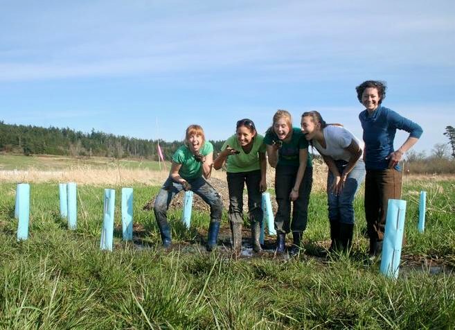
Enjoying the mud at Beaverton Marsh!
effects on the marine ecosystems. It’s something that isn’t thought of that much, with the exception of direct dumping into the environment and potential contamination of groundwater. But it is a concept that deserves more attention. This terrestrial impact has been the focus of our service projects this year, and rightfully so. Last week, we helped work on the enhancement and restoration of Beaverton Marsh. Over the years, the invasive reed canary grass has taken over the wetland, which has fallen victim to agricultural overuse. The restoration project aims to help restore native species and increase the diversity of the marsh. So for a couple of hours we all sloshed around in the mud and put plant protectors and mulch on plants that had been previously planted. It was hard work, but well worth the effort. Plus, it was a GORGEOUS day, which made it very enjoyable!
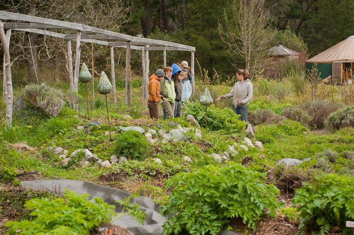
Last Friday we spent the day helping out on an organic local farm. We toured the farm and learned
Sweet Earth Farms- photo by Carlos Sanchez
a bit about organic farming on the island. We talked about permaculture, which is a type of agriculture that tries to model natural processes in nature. For example, there is a heavy focus on the use of perennial plants over annual plants (which need to be planted every year). The majority of plants found in the wild are perennials, which have a very stable root system. These long, deep roots absorb nutrients more efficiently, and so generally require less maintenance than annuals, and don’t deplete the topsoil as much. For more information on the use of perennials vs. annuals, check out this article from National Geographic.
Now you might be wondering what all of this really has to do with whales. It turns out, a lot! The three main threats to the southern resident killer whales were listed as being: 1) Prey availability, 2) Vessel noise, and 3) Toxins. The terrestrial environment can have a large effect on both prey availability and toxins. Degradation of the spawning environments of Chinook salmon can limit the returns of the fish back to the ocean. These rivers are easily affected by humans and agriculture. Cattle and other livestock can erode the river and stream banks and the removal of riparian vegetation leads to decreased shelter from predators (provided by shade) and increased temperatures that could rise to undesirable levels for the cold-loving salmon. Agricultural runoff creates an influx of nutrients that can lead to eutrophication and decreased oxygen content in water bodies. Dams create barriers to salmon migration to spawning areas. All of these lead to less fish for the killer whales to eat.
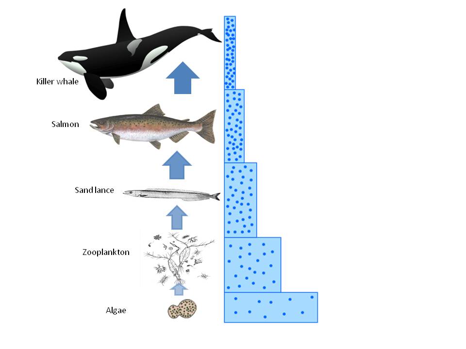
Toxins also pose a huge threat to the killer whales. High on the trophic pyramid, the killer whales suffer from the bioaccumulation of chemicals (see diagram at right). High levels of DDT, PCBs, and PBDEs have been found in killer whales. These are all organic chemicals that don’t breakdown well, leading to relatively high levels in the marine environment, even for the now illegal DDT. Indeed, many pesticides are a problem. Kwiaht in 2008 found that pyrethroid pesticide levels in the San Juan County waters averaged 1-2 parts per billion, with much higher levels in some areas. Levels of 1 part per billion are known to be toxic to salmonids. Surfactants, which are chemicals used to mix water and oil, are present in nearly every man-made product. The Friday Harbor Aquarium found lethal levels of surfactants in the surrounding water.
All of these toxins come from the terrestrial environment. It is important to be conscious of what we’re pouring down the drain or dumping outside. The San Juan Islands were heavily glaciated in the last ice age, which has resulted in very thin soils in many areas. Soil typically helps to filter groundwater. This decreased filtration can lead to increased runoff of chemicals to the marine environment. It’s important to be conscious of what we’re pouring down the drain or dumping outside. Try to minimize the amount of chemicals poured down the drain. Take care of your septic system to help prevent leakage. Restoration projects help bring back native species which help balance the ecosystem. Sustainable agricultural processes help reduce the runoff of toxic pesticides and other chemicals. So be cautious, be aware, and help protect these iconic animals!
Today NOAA finally issued a new rule that will govern how boats interact with endangered southern resident killer whales in 2011, starting in early May. The big news is that the legal approach distance has been doubled from 100 yards to 200 yards and the proposed “no-go” zone along the west side of San Juan Island will not be implemented.
The rule will go into affect 30 days after the date of the official Federal Register notice. The NOAA web site suggests the notice publication date is not yet known, but will presumably be today or within the next couple days:
Apr. 8, 2011: The Northwest Region announced final regulations to protect killer whales in Washington State from the effects of various vessel activities. There may be minor changes once the rule officially files.
Here’s what the Q&A document says about how and why the final rule differed from the proposed rule and suggested conservation actions:
The proposed rule included a no-go zone along the west side of San Juan Island that boats would not be allowed to enter from May through September. The no-go zone was not adopted as part of the final rule. During the public comment period, we received a large number of comments specific to the no-go zone including new speed zone alternatives, different exceptions, and questions about the economic impacts of a no-go zone. We’ve decided to gather additional information and conduct further analysis and public outreach on the concept of a no-go zone, which may be part of a future rulemaking.
The “Be Whale Wise” guidelines have not yet been updated to reflect the new rule at http://www.bewhalewise.org/ That will presumably be rectified shortly, as the management, whale watching, research, and stewardship communities rally around the vast educational outreach that will be necessary to promulgate the new rules efficiently during the 2011 boating season.
A key issue this season will be how many resources can be mobilized for both education and enforcement. NOAA is forecasting a gloomy funding environment generally for their 2011-2012 fiscal year. Does the cancellation of the normally-annual survey for southern resident killer whales along the outer Washington coast by NWFSC suggest there will be even fewer NOAA enforcement agents trained and monitoring boat-orca interactions this summer? Will Soundwatch and Straitwatch be adequately funded? Given the state of the WA State budget, it seems highly unlikely that WDFW or the San Juan County Sheriff will increase their training or monitoring presence…
Thanks to Jenny Atkinson of The Whale Museum for the notice of the announcement today.
This Sunday (10/10/10) Beam Reach will be joining thousands of other 350.org activists around the globe to do something about global warming. If you’d like to help reduce the concentration of carbon dioxide in the atmosphere from its current level, 390 parts per million (ppm), back down to what scientists say is a safe limit (350 ppm), then use this map to find a local event that interests you.
If you can’t find an inspiring action to join this weekend, we recommend that you use this cool website to make your home more efficient. Not only does the site provide a prioritized list of actions you can take to reduce your carbon footprint, but also it shows you how you can save money through conservation. It turns out green is gold!
We who live in Washington State have a special obligation to reduce our energy use. Not only do many of us contribute to global warming by burning natural gas or fuel oil to get through the cold months, but our electricity use is directly impacting the hunger level of one of our most cherished regional icons: the killer whale. You might think that because Washington Public Utility Districts get 82% of our electricity from hydropower, that we’re pioneers of sustainable energy use in America.
The problem is that we’ve recently learned that our local orcas love eating chinook salmon, particularly the big fish that return to the Columbia and Fraser Rivers. Unfortunately, the same dams that provide our power are preventing the recovery of chinook populations on the Columbia and Snake Rivers. Reducing our energy use in Washington is a direct way to allow more water to be spilled over dams in the short term (increasing smolt survival) and more dams to be removed in the long term (giving adult salmon easier access to pristine habitat). With plenty of salmon to power them through the winter, perhaps our orcas could recover from their current ~85 animals to their historic 150, bringing the combined (southern and northern) resident killer whale population to 350 itself!
On land at Beam Reach headquarters in Seattle, we’re always humbled when the students at sea report their water and energy use levels. Their typical daily water usage is only 2.5 gallons/person/day! In comparison, in our typical residential house we use 40 gallons/person/day.  All energy on the Beam Reach boat comes from biodiesel, and the students’ usage is about 0.5 gallons/person/day.
At sea, we’ll be continuing our efforts to practice sustainability science. We’ll be powering our studies of endangered killer whales with biodiesel bought from local supplier Island Petroleum Services.  Our captain, Todd Shuster, encourages us to burn biodiesel instead of fossil diesel in the 42′ sailing catamaran, Gato Verde, that has a nearly-silent Prius-like hybrid electric propulsion system that enables us to listen to the orcas as we move with them. We’ll also be discussing the science and ethics of deriving liquid fuels from oceanic plants while filtering some plankton and taking a first stab at extracting their oil for conversion to biodiesel.
If you’re not a home owner or can’t modify your living space, another action we recommend is to try cooking a meat-free meal this Sunday. Food production from farm to fork is responsible for between 20-30 percent of global green house gas emissions. Over your vegetarian meal you can discuss joining the meat-free Mondays movement, a way to make small changes in your life that can make a big difference for the planet.
There are many ways to lower CO2 levels and many questions yet to answer. We hope you’ll join us in considering them creatively while taking a few practical steps forward this weekend.
I got blisters on my fingers… and by fingers, I mean toes. My feet have never been so beat up in my entire life, but I can safely say that I sacrificed their happiness for a worthy cause. On Saturday, Libby and I walked from the marina in Sidney, British Columbia all the way to the parliament building in Victoria.
Libby walking
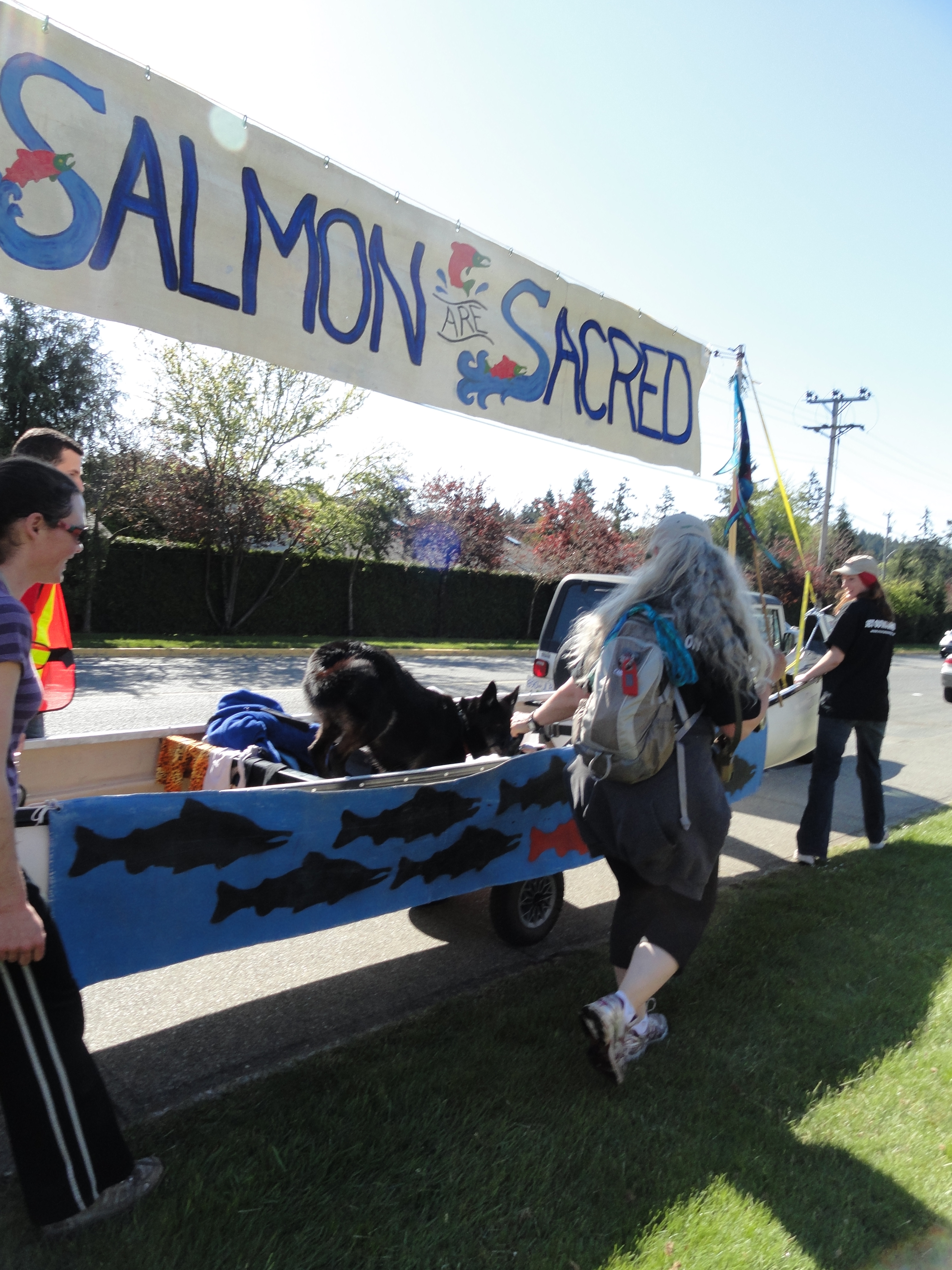
We walked approximately 18 miles with hundreds of other people as part of the Get Out Migration, a march to raise awareness about open-pen fish farms led by a woman named Alexandra Morton. She has lived in the Broughton Archipelago for more than twenty years, researching the Northern resident killer whale community and, more recently, the effects of open-pen fish farms on the wild salmon populations. After ten years of working to eradicate Norwegian fish farms from the area, Alexandra organized a three-week walk from the Northernmost to Southernmost tip of Vancouver Island to spread the word about their negative impact on local communities and ecosystems. During a trip to Vancouver Island a few years ago, my father bought me Alexandra’s book, Listening to Whales. I did not read it until last summer, when I was living at a remote research station off the cost of Maine. Her narrative about studying killer whales and her depiction of life as a field scientist was formative for me – since then, I have dreamed of meeting Alexandra Morton. When I heard that she was due to walk into Victoria while I was right across the water, I decided then and there that I had to walk with her. After much logistical planning, Libby and I pinned down a ride and set out for Sidney. Because we had to clear customs, we missed the start of the walk at 8 am, so the beginning of our journey was fairly rushed. Walking briskly through the Sidney suburbs without any sight of Alexandra and her entourage, Libby and I started to wonder if we’d be walking all the way to Victoria alone. Just as we were beginning to contemplate hitchhiking, a car pulled up beside us. “Hey, are you guys trying to catch up to the migration?â€Â A young woman named Megan, who turned out to be none other than Alex Morton’s assistant, opened her car door and ushered us inside. “I know migrators when I see them!†she said. Five minutes later, we came upon a train of cars, signaling the back of the migration pack. A woman with long, wispy white hair came into view, and my eyes widened. I was way too sweaty and frazzled to be thrust into the presence of Alexandra Morton already! Libby and I thanked Megan for saving us many uncomfortable miles of walking and started down the road, trailing Alex’s heels and wondering what to do next. Turns out my body is not too keen on the idea of walking 18 miles, so for the majority of our migration to Victoria, I was solely focused on putting one foot in front of the other. Because of this, I did not get the heart-to-heart with Alex I had imagined, but simply being in her presence and taking part in this massive culmination of her efforts was enough for me. After a long day of trekking down Highway 17, we entered Victoria, greeted by a huge group of supporters. The final 1 km walk to the parliament building was spectacular – thousands of people flooded the streets, marching to the beat of the First Nations’ drum and shouting to spectators.
At the Parliament Building
It became evident to me that this is an issue that affects all of British Columbia’s citizens in different ways, but it is undeniable that the effects are uniformly negative. Libby and I collapsed on the parliament building lawn, ready to yank our shoes off and douse ourselves with cold water. The wide range of speakers at the final migration event, from First Nations chiefs to commercial fishermen, spoke of the cross-cultural concerns fish farms have raised. There were so many people crammed onto the lawn that we could not even see the stage, but it was enough just to be able to sit and listen. Alexandra was the last to speak; I had not lost all hope of meeting her, so I tried to keep one eye on her as she snaked back through the crowd amidst roaring applause. Libby pointed. “There she is!â€Â We knew this was the last chance we would get, so we pushed forward until we were standing right in front of her. As this was the end of Alex’s very long journey, I didn’t want to goad her into taking a photo with me or signing my book. I just wanted to say hello, so that’s what I did. Libby somehow managed to snap a candid photo of this moment (she’s amazing!), and I am so glad she did. Like I said, the blisters were well worth the pain.
Meeting Alexandra (Libby’s picture)
To learn more about the Get Out Migration, click here


 Twitter
 LinkedIn
 Facebook